机器学习学习笔记（第一周）-斯坦福大学

第一周

What is Machine Learning?

What is Machine Learning?
Two definitions of Machine Learning are offered. Arthur Samuel described it as: “the field of study that gives computers the ability to learn without being explicitly programmed.” This is an older, informal definition.

Tom Mitchell provides a more modern definition: “A computer program is said to learn from experience E with respect to some class of tasks T and performance measure P, if its performance at tasks in T, as measured by P, improves with experience E.”

Example: playing checkers.

E = the experience of playing many games of checkers

T = the task of playing checkers.

P = the probability that the program will win the next game.

In general, any machine learning problem can be assigned to one of two broad classifications:

Supervised learning and Unsupervised learning.

---

Supervised Learning

在正式定义有监督学习之前，不妨先来看一个例子：

上图是收集到的美国房价数据，横轴是平方英尺，纵轴是价格：千美元。
现在假设一位朋友需要卖房，他的房子面积是750平方英尺，但是我们并没有收集到750 feet^2 的数据，那么我们该如何估算该房价呢？

Unsupervised Learning

先来回想上次所讲的监督学习中的数据集，每个样本都已经被标明为正样本或者负样本，即良性或恶性肿瘤。因此，对于监督学习中的每一个样本，我们都已经被清楚地告知了什么是所谓的正确答案。

在无监督学习中，我们用的数据会和监督学习里的看起来不太一样。在无监督学习中，没有属性或标签这一概念，也就是说所有的数据都是一样的，没有区别。
所以在无监督学习中，我们只有一个数据集，没人告诉我们该怎么做，我们也不知道，每个数据点究竟是什么意思。相反它只告诉我们：现在有一个数据集，你能在其中找到某种结构吗？
对于给定的数据集，无监督学习算法可能判定，该数据集包含两个不同的聚类。
Unsupervised Learning
Unsupervised learning allows us to approach problems with little or no idea what our results should look like. We can derive structure from data where we don’t necessarily know the effect of the variables.

We can derive this structure by clustering the data based on relationships among the variables in the data.

With unsupervised learning there is no feedback based on the prediction results.

Example:

Clustering: Take a collection of 1,000,000 different genes, and find a way to automatically group these genes into groups that are somehow similar or related by different variables, such as lifespan, location, roles, and so on.

Non-clustering: The “Cocktail Party Algorithm”, allows you to find structure in a chaotic environment. (i.e. identifying individual voices and music from a mesh of sounds at a cocktail party).

Model Representation
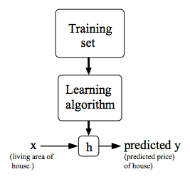
To establish notation for future use, we’ll use x(i) to denote the “input” variables (living area in this example), also called input features, and y(i)to denote the “output” or target variable that we are trying to predict (price). A pair (x (i) ,y (i) ) is called a training example, and the dataset that we’ll be using to learn—a list of m training examples (x(i),y(i));i=1,…,m—is called a training set. Note that the superscript “(i)” in the notation is simply an index into the training set, and has nothing to do with exponentiation. We will also use X to denote the space of input values, and Y to denote the space of output values. In this example, X = Y = ℝ.

To describe the supervised learning problem slightly more formally, our goal is, given a training set, to learn a function h : X → Y so that h(x) is a “good” predictor for the corresponding value of y. For historical reasons, this function h is called a hypothesis. Seen pictorially, the process is therefore like this:

When the target variable that we’re trying to predict is continuous, such as in our housing example, we call the learning problem a regression problem. When y can take on only a small number of discrete values (such as if, given the living area, we wanted to predict if a dwelling is a house or an apartment, say), we call it a classification problem.

Cost Function
We can measure the accuracy of our hypothesis function by using a cost function. This takes an average difference (actually a fancier version of an average) of all the results of the hypothesis with inputs from x’s and the actual output y’s.

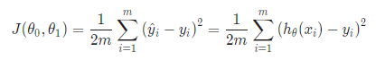
If we try to think of it in visual terms, our training data set is scattered on the x-y plane. We are trying to make a straight line (defined by hθ (x)) which passes through these scattered data points.
Our objective is to get the best possible line. The best possible line will be such so that the average squared vertical distances of the scattered points from the line will be the least. Ideally, the line should pass through all the points of our training data set. In such a case, the value of J(θ 0 ,θ 1 ) will be 0. The following example shows the ideal situation where we have a cost function of 0.

When θ1=1, we get a slope of 1 which goes through every single data point in our model. Conversely, when θ1=0.5, we see the vertical distance from our fit to the data points increase.

This increases our cost function to 0.58. Plotting several other points yields to the following graph:

Thus as a goal, we should try to minimize the cost function. In this case, θ1=1 is our global minimum.

Cost Function - Intuition II
A contour plot is a graph that contains many contour lines. A contour line of a two variable function has a constant value at all points of the same line. An example of such a graph is the one to the right below.

Taking any color and going along the ‘circle’, one would expect to get the same value of the cost function. For example, the three green points found on the green line above have the same value for J(θ0,θ1) and as a result, they are found along the same line. The circled x displays the value of the cost function for the graph on the left when θ0= 800 and θ1= -0.15. Taking another h(x) and plotting its contour plot, one gets the following graphs:

When θ0= 360 and θ1= 0, the value of J(θ0,θ1) in the contour plot gets closer to the center thus reducing the cost function error. Now giving our hypothesis function a slightly positive slope results in a better fit of the data.

The graph above minimizes the cost function as much as possible and consequently, the result of θ1 and θ0 tend to be around 0.12 and 250 respectively. Plotting those values on our graph to the right seems to put our point in the center of the inner most ‘circle’.

Gradient Descent
So we have our hypothesis function and we have a way of measuring how well it fits into the data. Now we need to estimate the parameters in the hypothesis function. That’s where gradient descent comes in.

Imagine that we graph our hypothesis function based on its fields θ0 ​and θ1 (actually we are graphing the cost function as a function of the parameter estimates). We are not graphing x and y itself, but the parameter range of our hypothesis function and the cost resulting from selecting a particular set of parameters.

We put θ0 on the x axis and θ1 on the y axis, with the cost function on the vertical z axis. The points on our graph will be the result of the cost function using our hypothesis with those specific theta parameters. The graph below depicts such a setup.

We will know that we have succeeded when our cost function is at the very bottom of the pits in our graph, i.e. when its value is the minimum. The red arrows show the minimum points in the graph.

The way we do this is by taking the derivative (the tangential line to a function) of our cost function. The slope of the tangent is the derivative at that point and it will give us a direction to move towards. We make steps down the cost function in the direction with the steepest descent. The size of each step is determined by the parameter α, which is called the learning rate.

For example, the distance between each ‘star’ in the graph above represents a step determined by our parameter α. A smaller α would result in a smaller step and a larger α results in a larger step. The direction in which the step is taken is determined by the partial derivative of J(θ0 ,θ1). Depending on where one starts on the graph, one could end up at different points. The image above shows us two different starting points that end up in two different places.

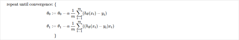
The gradient descent algorithm is:

repeat until convergence:

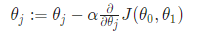
where
j=0,1 represents the feature index number.

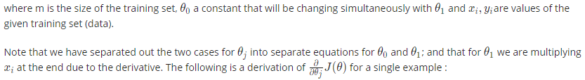
At each iteration j, one should simultaneously update the parameters θ1,θ2,…,θn. Updating a specific parameter prior to calculating another one on the j(th) iteration would yield to a wrong implementation.

Gradient Descent Intuition






Gradient Descent For Linear Regression
When specifically applied to the case of linear regression, a new form of the gradient descent equation can be derived. We can substitute our actual cost function and our actual hypothesis function and modify the equation to :



The point of all this is that if we start with a guess for our hypothesis and then repeatedly apply these gradient descent equations, our hypothesis will become more and more accurate.

So, this is simply gradient descent on the original cost function J. This method looks at every example in the entire training set on every step, and is called batch gradient descent. Note that, while gradient descent can be susceptible to local minima in general, the optimization problem we have posed here for linear regression has only one global, and no other local, optima; thus gradient descent always converges (assuming the learning rate α is not too large) to the global minimum. Indeed, J is a convex quadratic function. Here is an example of gradient descent as it is run to minimize a quadratic function.

The ellipses shown above are the contours of a quadratic function. Also shown is the trajectory taken by gradient descent, which was initialized at (48,30). The x’s in the figure (joined by straight lines) mark the successive values of θ that gradient descent went through as it converged to its minimum.

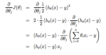
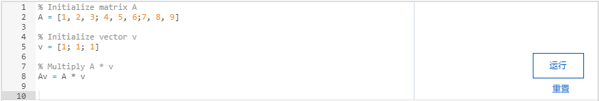
Matrices and Vectors