einops可视化理解

最近在看vit_pytorch代码，看到里面有很多地方用到einops来对tensor操作，本实验结合这篇博客内容和自己一些尝试。
代码colab链接

import einops
import matplotlib.pyplot as plt
import numpy as np

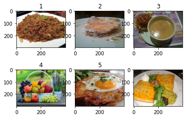
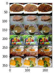
读取一个文件夹下图片生成一个batch

from PIL import Image
import os

images = [np.array(Image.open('./images/'+file_name).resize((400, 300))) for file_name in os.listdir('./images') if file_name.endswith('.jpg')]
images = (np.array(images)/255.0)

print(images.shape)
print(images.dtype)

col = 3
row = int(len(imges)/col)

for i in range(row):
    for j in range(col):
        index = i*col+j
        plt.title(index)
        plt.subplot(row, col, index+1) 
        plt.imshow(images[index])
plt.show()

(6, 300, 400, 3)
float64

Rearrange

from einops import rearrange

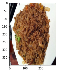
switch dimension

print(images.shape)
image = rearrange(images[0], 'h w c -> w h c') # 转置，对角线对称
print(image.shape)
plt.imshow(image)
plt.show()

(6, 300, 400, 3)
(400, 300, 3)

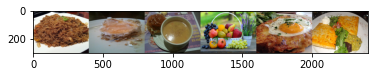
merge dimension

print(images.shape)
image = rearrange(images, 'b h w c -> (b h) w c') # 在h维度合并
print(image.shape)
plt.imshow(image)
plt.show()

(6, 300, 400, 3)
(1800, 400, 3)

print(images.shape)
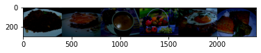
image = rearrange(images, 'b h w c -> h (b w) c') # 在w维度合并
print(image.shape)
plt.imshow(image)
plt.show()

(6, 300, 400, 3)
(300, 2400, 3)

print(images.shape)
image = rearrange(images, '(b1 b2) h w c -> b1 b2 h w c ', b1=2) # 先分成2组，每组3张是自动计算得到
print(image.shape)
image = rearrange(image, 'b1 b2 h w c  -> b1 h (b2 w) c ') # 每组先合并
print(image.shape)
image = rearrange(image, 'b1 h w c  -> (b1 h) w c ') # 合并每组
print(image.shape)

plt.imshow(image)
plt.show()

(6, 300, 400, 3)
(2, 3, 300, 400, 3)
(2, 300, 1200, 3)
(600, 1200, 3)

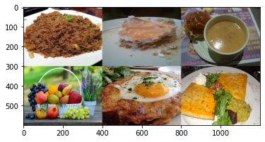
或者一次性完成

print(images.shape)
image = rearrange(images, '(b1 b2) h w c -> (b1 h) (b2 w) c',  b1=2) # b1=2时，b2=3，在h维度合3张图并产生2组，然后在w维度上合并2组，
plt.imshow(image)
plt.show()

(6, 300, 400, 3)

Reduce

from einops import reduce

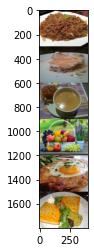
average over channel

print(images.shape)
image = reduce(images, 'b h w c -> b h w', reduction='mean') # 在c维度上求均值
print(image.shape)
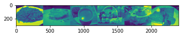
image = rearrange(image, 'b h w -> h (b w)') # 在w维度合并
print(image.shape)

plt.imshow(image)
plt.show()

plt.imshow(images[0].mean(-1))
plt.show()

(6, 300, 400, 3)
(6, 300, 400)
(300, 2400)

注：为什么plt单通道不是灰度图

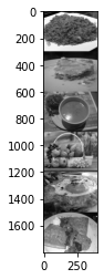
reduce操作包含了rearrange操作，比如下面使用reduce实现了在c维度上求均值外，还实现了rearrange排列的功能，所以只需一句pattern

print(images.shape)
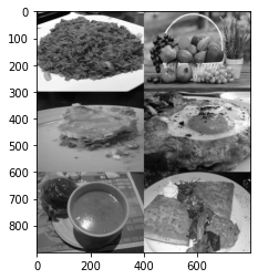
image = reduce(images, '(b1 b2) h w c -> (b2 h) (b1 w)', reduction='mean', b1=2) # b1=2时，b2=3，在h维度合3张图并产生2组，然后在w维度上合并2组，
plt.imshow(image, cmap='gray')
plt.show()

(6, 300, 400, 3)

average over batch

# average over batch
print(images.shape)
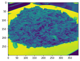
image = reduce(images, 'b h w c -> h w c', reduction='mean') # 在batch上求平均
print(image.shape)

plt.imshow(image)
plt.show()

(6, 300, 400, 3)
(300, 400, 3)

mean/max/min-pooling

print(images.shape)
image_mean = reduce(images, 'b (h h2) (w w2) c -> (b h) w c', reduction='mean', h2=5, w2=5) # h 和 w 变小，实现5 x 5 的均值池化
print(image_mean.shape)
image_max = reduce(images, 'b (h h2) (w w2) c -> (b h) w c', reduction='max', h2=5, w2=5) # h 和 w 变小，实现5 x 5 的最大池化
print(image_max.shape)
image_min = reduce(images, 'b (h h2) (w w2) c -> (b h) w c', reduction='min', h2=5, w2=5) # h 和 w 变小，实现5 x 5 的最小池化
print(image_min.shape)

image = np.array([image_mean, image_max, image_min])
print(image.shape)

image = rearrange(image, 'b h w c -> h (b w) c') # 在w维度合并
print(image.shape)

plt.imshow(image)
plt.show()

(6, 300, 400, 3)
(360, 80, 3)
(360, 80, 3)
(360, 80, 3)
(3, 360, 80, 3)
(360, 240, 3)

global average pooling

print(images.shape)
image = reduce(images, 'b h w c -> b c', 'mean')
print(image.shape)
print(image)

(6, 300, 400, 3)
(6, 3)
[[0.60353327 0.48071248 0.39087559]
 [0.4849948  0.45346219 0.41585203]
 [0.43090971 0.38947967 0.31965755]
 [0.48734565 0.50724111 0.34352359]
 [0.56760291 0.43742605 0.32223343]
 [0.66422222 0.56174487 0.32173595]]

Repeat

from einops import repeat

print(images.shape)
image = reduce(images, 'b h w c -> b h w', 'mean')
print(image.shape)
image = repeat(image, 'b h w -> (b h) w c', c=3)# copy along a new axis 
print(image.shape)

plt.imshow(image) # 3通道颜色一样
plt.show()

(6, 300, 400, 3)
(6, 300, 400)
(1800, 400, 3)

Addition or removal of axes

print(images.shape)
image = rearrange(images, 'b h w c -> b 1 h w 1 c') # functionality of numpy.expand_dims
print(image.shape)
image = rearrange(image, 'b 1 h w 1 c -> (b h) w c') # functionality of numpy.squeeze
print(image.shape)

plt.imshow(image)
plt.show()

(6, 300, 400, 3)
(6, 1, 300, 400, 1, 3)
(1800, 400, 3)

difference

print(images.shape)
image = reduce(images, 'b h w c -> b () () c', 'max') -  images # 计算每张图最大值，然后计算与原图差值
print(image.shape)
image = rearrange(image, 'b h w c -> h (b w) c')
print(image.shape)

plt.imshow(image)
plt.show()

(6, 300, 400, 3)
(6, 300, 400, 3)
(300, 2400, 3)

flatten

print(images.shape)
image = rearrange(images, 'b h w c -> b (h w c)') # 1维展开
print(image.shape)
print(image)

(6, 300, 400, 3)
(6, 360000)
[[0.11372549 0.1254902  0.10588235 ... 0.07058824 0.03529412 0.05490196]
 [0.03921569 0.03921569 0.         ... 0.44705882 0.5254902  0.52941176]
 [0.45098039 0.32156863 0.29019608 ... 0.17254902 0.16078431 0.1254902 ]
 [0.30196078 0.2627451  0.11764706 ... 0.16078431 0.18431373 0.20784314]
 [0.49411765 0.5372549  0.29019608 ... 0.7254902  0.67843137 0.62352941]
 [0.14901961 0.14509804 0.13333333 ... 0.82745098 0.83137255 0.81176471]]

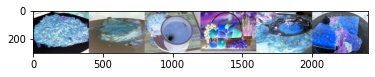
mean-normalization

print(images.shape)
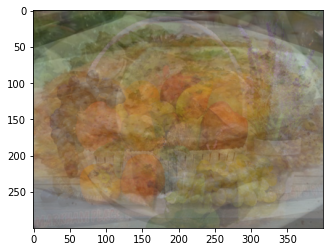
image = images - reduce(images, 'b h w c -> b 1 1 c', 'mean')
print(image.shape)

image = rearrange(image, 'b h w c -> h (b w) c')
print(image.shape)

plt.imshow(image)
plt.show()

Clipping input data to the valid range for imshow with RGB data ([0..1] for floats or [0..255] for integers).


(6, 300, 400, 3)
(6, 300, 400, 3)
(300, 2400, 3)

patch

print(images.shape)
image = rearrange(images, 'b (h p_h) (w p_w) c -> b (h w) p_h p_w c', p_h = 150, p_w = 200) # 一张图划分为3个patch
print(image.shape)

image = rearrange(image, 'b l p_h p_w c ->  (l p_h) (b p_w) c')
print(image.shape)

plt.imshow(image)
plt.show()

(6, 300, 400, 3)
(6, 4, 150, 200, 3)
(600, 1200, 3)

参考

pytorch-examples