(最新！)CRU数据集：1901~2024年全球降水、气温、潜在蒸散发、气压、云量等气象要素（附R处理代码）

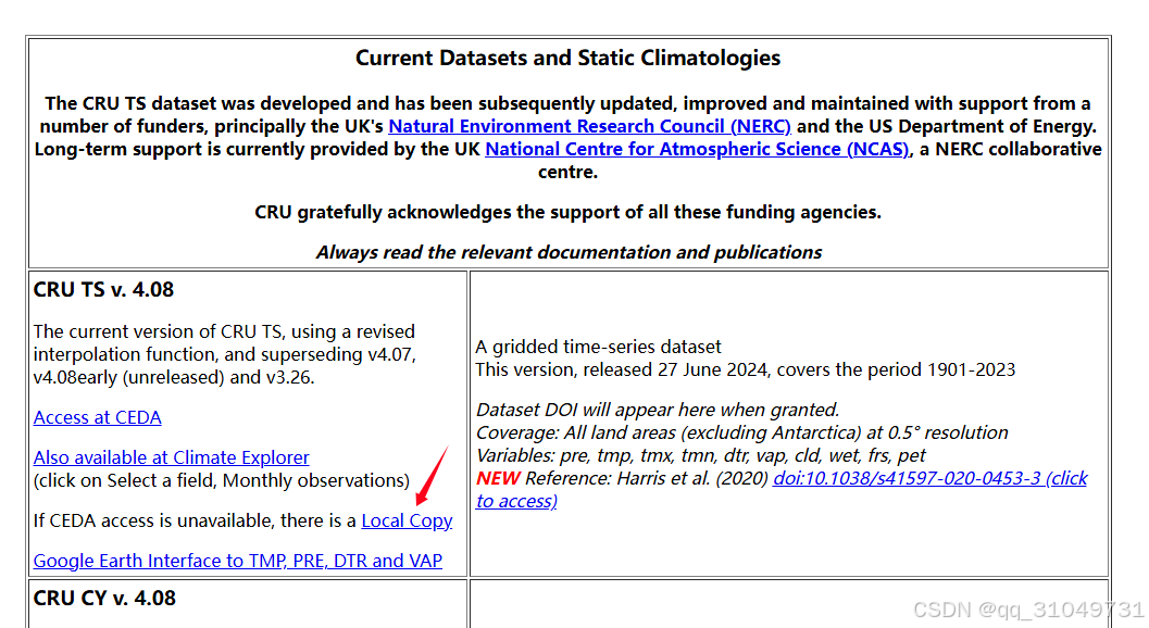
CRU 是目前使用最广泛的气候数据集之一，由英国国家大气科学中心 (NERC Centres for Atmospheric Science (UK)，NCAS) 制作。CRU TS 提供全球1901 年至 2024 年覆盖陆地表面的 0.5° 分辨率的月度数据。数据集主要的气象因素有：温度（平均值、最小值、最大值和昼夜温差）、降水量（总量，雨天数）、湿度（如蒸气压）、霜天数、云量和潜在的蒸腾作用。

目前已经更新为：CRU TS v. 4.08，如下图：

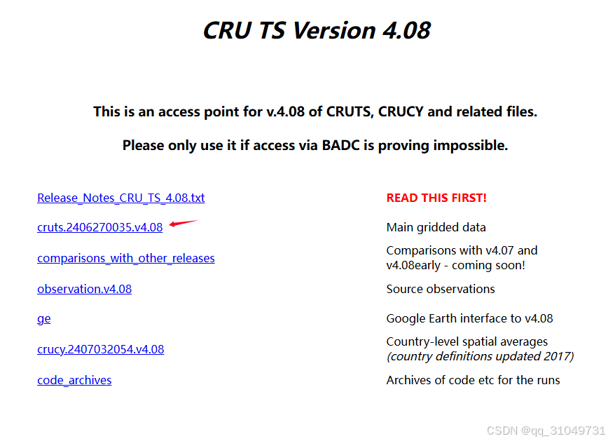
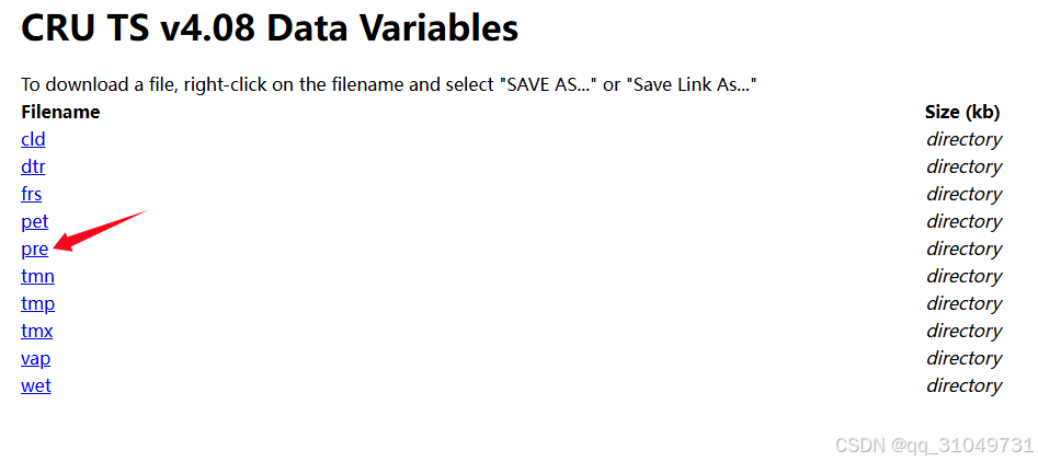
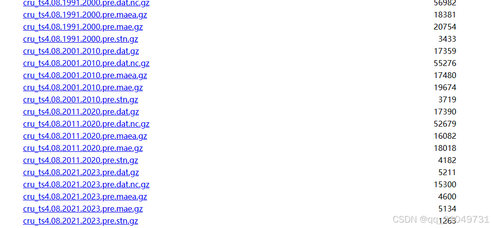
下载地址：https://crudata.uea.ac.uk/cru/data/hrg/

附分析方法：（R软件代码）

============

# 加载必要的包
library(ncdf4)
library(raster)
library(ggplot2)
library(sf)
library(ggspatial)
library(ggthemes)

# 1. 读取NetCDF数据
data <- "./cru_ts4.08.1901.2023.pre.dat.nc"
nc_data <- nc_open(data)

# 读取变量
temp1 <- ncvar_get(nc_data, "pre")
time1 <- ncvar_get(nc_data, "time")
lat1 <- ncvar_get(nc_data, "lat")
lon1 <- ncvar_get(nc_data, "lon")

nc_close(nc_data)

# 2. 提取特定时间段的数据（2023年）
# 假设时间维度是月度数据，1465:1476对应2023年的12个月
temp1 <- temp1[, , 1465:1476]

# 3. 计算总降水量
temp2 <- apply(temp1, 1:2, sum)

# 4. 创建空间数据框
raster_data <- raster(t(temp2), xmn=min(lon1), xmx=max(lon1), ymn=min(lat1), ymx=max(lat1))
raster_data <- flip(raster_data, direction = "y") # 翻转纬度

# 5. 绘制降水分布图
# 创建地图数据
china_provinces <- st_read("./China_Province.shp")
ten_line <- st_read("./10line.shp")

# 绘制主图
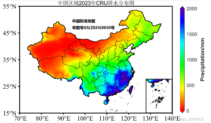
ggplot() +
  annotation_custom(rasterGrob(raster_data, interpolate = TRUE), 
                    xmin = min(lon1), xmax = max(lon1), ymin = min(lat1), ymax = max(lat1)) +
  geom_sf(data = china_provinces, color = "black", fill = NA) +
  geom_sf(data = ten_line, color = "black") +
  scale_fill_gradientn(colors = rainbow(7), limits = c(0, 2000)) +
  theme_map() +
  theme(axis.text.x = element_text(size = 12),
        axis.text.y = element_text(size = 12),
        axis.title = element_text(size = 12),
        legend.position = "right",
        legend.text = element_text(size = 10),
        legend.title = element_text(size = 10, face = "bold")) +
  labs(fill = "Precipitation (mm)",
       title = "中国区域2023年CRU降水分布图") +
  coord_cartesian(xlim = c(70, 140), ylim = c(15, 55)) +
  annotation_scale(location = "bl", width_hint = 0.5) +
  annotation_north_arrow(location = "bl", which_north = "true", 
                         pad_x = unit(0.5, "in"), pad_y = unit(0.5, "in"),
                         style = north_arrow_fancy_orienteering)

# 6. 添加南海小图
# 创建南海小图
south_china_sea <- ggplot() +
  annotation_custom(rasterGrob(raster_data, interpolate = TRUE), 
                    xmin = min(lon1), xmax = max(lon1), ymin = min(lat1), ymax = max(lat1)) +
  geom_sf(data = china_provinces, color = "black", fill = NA) +
  geom_sf(data = ten_line, color = "black") +
  scale_fill_gradientn(colors = rainbow(7), limits = c(0, 2000)) +
  theme_void() +
  coord_cartesian(xlim = c(105, 124), ylim = c(0, 24))

# 组合主图和小图
library(grid)
library(gridExtra)

main_plot <- ggplot_gtable(ggplot_build(last_plot()))
small_plot <- ggplot_gtable(ggplot_build(south_china_sea))

# 调整小图位置
small_plot$vp <- viewport(x = 0.66, y = 0.25, width = 0.2, height = 0.2)

grid.draw(main_plot)
grid.draw(small_plot)

======