


棒球运动员的身高、体重的特点
作者获得了一份从1820到1995年出生的棒球运动员的身体数据。这里我对各地运动员的身高、体重情况以及他们随着时间的变化,以及它们和运动员寿命的关系情况感兴趣。接下来,我将对这些进行分析
提出问题:
1.运动员的出生区域分布
2.运动员的身高、体重随出生年份的变化
3.运动员的寿命与身高、体重的关系

这里,运动员的身高、体重是因变量,年份、城市是自变量
#导入数据库

# -*- coding: utf-8 -*-
import numpy as np
import pandas as pd
import matplotlib.pyplot as plt
import seaborn as sns
from __future__ import division
%matplotlib inline
导入数据
def read_csv(filename):
    file=filename
    data=pd.read_csv(file)
    return(data)
player_df=read_csv('Master.csv')
#stars_df=read_csv('AllstarFull.csv')
让我们先来看一下导入的数据的结构
player_df.head()| playerID | birthYear | birthMonth | birthDay | birthCountry | birthState | birthCity | deathYear | deathMonth | deathDay | ... | nameLast | nameGiven | weight | height | bats | throws | debut | finalGame | retroID | bbrefID | |
|---|---|---|---|---|---|---|---|---|---|---|---|---|---|---|---|---|---|---|---|---|---|
| 0 | aardsda01 | 1981.0 | 12.0 | 27.0 | USA | CO | Denver | NaN | NaN | NaN | ... | Aardsma | David Allan | 220.0 | 75.0 | R | R | 2004/4/6 | 2015/8/23 | aardd001 | aardsda01 |
| 1 | aaronha01 | 1934.0 | 2.0 | 5.0 | USA | AL | Mobile | NaN | NaN | NaN | ... | Aaron | Henry Louis | 180.0 | 72.0 | R | R | 1954/4/13 | 1976/10/3 | aaroh101 | aaronha01 |
| 2 | aaronto01 | 1939.0 | 8.0 | 5.0 | USA | AL | Mobile | 1984.0 | 8.0 | 16.0 | ... | Aaron | Tommie Lee | 190.0 | 75.0 | R | R | 1962/4/10 | 1971/9/26 | aarot101 | aaronto01 |
| 3 | aasedo01 | 1954.0 | 9.0 | 8.0 | USA | CA | Orange | NaN | NaN | NaN | ... | Aase | Donald William | 190.0 | 75.0 | R | R | 1977/7/26 | 1990/10/3 | aased001 | aasedo01 |
| 4 | abadan01 | 1972.0 | 8.0 | 25.0 | USA | FL | Palm Beach | NaN | NaN | NaN | ... | Abad | Fausto Andres | 184.0 | 73.0 | L | L | 2001/9/10 | 2006/4/13 | abada001 | abadan01 |
5 rows × 24 columns
下面是数据中表头的含义:
1.playerID       A unique code asssigned to each player.  The playerID links
             the data in this file with records in the other files.
2.birthYear      Year player was born
3.birthMonth     Month player was born
4.birthDay       Day player was born
5.birthCountry   Country where player was born
6.birthState     State where player was born
7.birthCity      City where player was born
8.deathYear      Year player died
9.deathMonth     Month player died
10.deathDay       Day player died
11.deathCountry   Country where player died
12.deathState     State where player died
13.deathCity      City where player died
14.nameFirst      Player's first name
15.nameLast       Player's last name
16.nameGiven      Player's given name (typically first and middle)
17.weight         Player's weight in pounds
18.height         Player's height in inches
19.bats           Player's batting hand (left, right, or both)
20.throws         Player's throwing hand (left or right)
21.debut          Date that player made first major league appearance
数据项目有很多,但我们只需要选手ID,出生年份、出生国家、城市等数据,这里将提取这些数据
data1_df=player_df[['playerID','birthYear','deathYear','birthCountry','birthState','birthCity','weight','height']]让我们看一下新数据的结构
data1_df.head()| playerID | birthYear | deathYear | birthCountry | birthState | birthCity | weight | height | |
|---|---|---|---|---|---|---|---|---|
| 0 | aardsda01 | 1981.0 | NaN | USA | CO | Denver | 220.0 | 75.0 |
| 1 | aaronha01 | 1934.0 | NaN | USA | AL | Mobile | 180.0 | 72.0 |
| 2 | aaronto01 | 1939.0 | 1984.0 | USA | AL | Mobile | 190.0 | 75.0 |
| 3 | aasedo01 | 1954.0 | NaN | USA | CA | Orange | 190.0 | 75.0 |
| 4 | abadan01 | 1972.0 | NaN | USA | FL | Palm Beach | 184.0 | 73.0 |
接下来让我们查看一下数据的摘要信息
data1_df.describe()| birthYear | deathYear | weight | height | |
|---|---|---|---|---|
| count | 18703.000000 | 9336.000000 | 17975.000000 | 18041.000000 |
| mean | 1930.664118 | 1963.850364 | 185.980862 | 72.255640 |
| std | 41.229079 | 31.506369 | 21.226988 | 2.598983 |
| min | 1820.000000 | 1872.000000 | 65.000000 | 43.000000 |
| 25% | 1894.000000 | 1942.000000 | 170.000000 | 71.000000 |
| 50% | 1936.000000 | 1966.000000 | 185.000000 | 72.000000 |
| 75% | 1968.000000 | 1989.000000 | 200.000000 | 74.000000 |
| max | 1995.000000 | 2016.000000 | 320.000000 | 83.000000 |
从摘要信息中可以看到,棒球运动员的平均身高为72.255英寸,分布在43英寸到83英寸之间;体重的波动范围为65-320磅,平均体重为185.98磅
让我们看一下是否存在数据缺失情况
data1_df.info()<class 'pandas.core.frame.DataFrame'>
RangeIndex: 18846 entries, 0 to 18845
Data columns (total 8 columns):
playerID 18846 non-null object
birthYear 18703 non-null float64
deathYear 9336 non-null float64
birthCountry 18773 non-null object
birthState 18220 non-null object
birthCity 18647 non-null object
weight 17975 non-null float64
height 18041 non-null float64
dtypes: float64(4), object(4)
memory usage: 1.2+ MB
可以看到,数据中体重、身高、出生年份、死亡年份数据信息不全。
其中,身高、体重数据将用前值补全,出生年份缺失的则需要将其剔除
#定义补全函数
def enfull_ave(letter):

    data1_df[letter].fillna(method='ffill')
#补全体重
enfull_ave('weight')
#补全身高
enfull_ave('height')
#剔除缺失数据
data1_df=data1_df.dropna(how='all')
现在,让我们对棒球运动员的国家分布和城市分布进行分析
#下面定义几个常用函数
# 按照name对运动员进行分组后,计算每组的人数
def player_count(data,name):
    return data.groupby(name)['playerID'].count()

def player_count_rate(data,name):

    b=player_count(data,name)

    a=data['playerID'].count()

    return b/a

# 输出饼图
def print_pie(group_data,title):
    group_data.plot.pie(title=title,figsize=(12, 12),autopct='%3.1f%%',startangle =90,legend=True)
# 输出柱状图
def print_bar(data,title):
    bar=data.plot.bar(title=title,width=10)
    for p in bar.patches:
        bar.annotate('%3.1f%%' % (p.get_height()*100), (p.get_x() * 1.005, p.get_height() * 1.005))
#输出折线图
def print_plot(data,name1,title):

    x=data.index
    y=data[name1]
    plt.figure(figsize=(12,6)) #创建绘图对象
    plt.plot(x,y,'ro',color="red",linewidth=1)   #在当前绘图对象绘图(X轴,Y轴,蓝色虚线,线宽度)
    plt.xlabel("year")
    plt.ylabel(name1)
    plt.title(title) #图标题
    plt.show()  #显示图
    plt.savefig("line.jpg") #保存图
接下来,让我们查看棒球运动员在各个国家的分布比例
player_count_rate(data1_df,'birthCountry').sort_values(ascending=False)birthCountry
USA 0.875730
D.R. 0.034119
Venezuela 0.018094
P.R. 0.013425
CAN 0.012947
Cuba 0.010506
Mexico 0.006261
Japan 0.003290
Panama 0.002918
Ireland 0.002653
United Kingdom 0.002600
Germany 0.002441
Australia 0.001486
South Korea 0.000902
Colombia 0.000902
Nicaragua 0.000743
Curacao 0.000743
V.I. 0.000637
Netherlands 0.000637
Taiwan 0.000584
Russia 0.000424
France 0.000424
Italy 0.000371
Bahamas 0.000318
Aruba 0.000265
Poland 0.000265
Austria 0.000212
Sweden 0.000212
Spain 0.000212
Czech Republic 0.000212
Jamaica 0.000212
Brazil 0.000159
Norway 0.000159
Saudi Arabia 0.000106
At Sea 0.000053
American Samoa 0.000053
Belgium 0.000053
Belize 0.000053
China 0.000053
Viet Nam 0.000053
Denmark 0.000053
Finland 0.000053
Greece 0.000053
Guam 0.000053
Honduras 0.000053
Indonesia 0.000053
Lithuania 0.000053
Philippines 0.000053
Singapore 0.000053
Slovakia 0.000053
Switzerland 0.000053
Afghanistan 0.000053
Name: playerID, dtype: float64
可以看到,棒球运动员来自50多个国家和地区。绝大多数棒球运动员的出生国家在美国,占比87.6%;比较高的有D.R.、Venezuela、P.R.、CAN、Cuba ,都达到了1%以上。接下来,让我们看一下美国运动员的州分布
#提取美国运动员数据
data_usa=data1_df[data1_df['birthCountry']=='USA']
#画饼图
print_pie(player_count_rate(data_usa,'birthState'),'The player rate about States')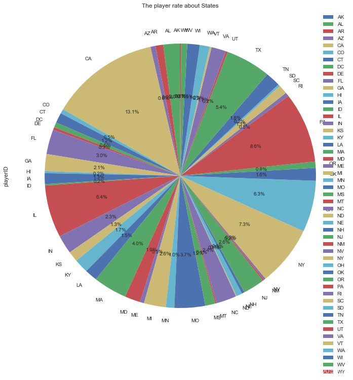
从这里可以看到,出生在CA的棒球运动员最多,占比为13%,其次为PA,为8.5%。排名前五的州为CA,PA,NY,IL,OH,有超过44%的美国棒球运动员在这些地方出生
让我们看一下各地棒球运动员的身高、体重情况吧
data2=data1_df[['birthCountry','birthState','height','weight']]
#按平均身高排序
data3=data2.groupby('birthCountry').mean().sort_values(by='height',ascending=False)
print '有%d个国家超过了平均水平'%(data3['height'][data3['height']>=data1_df['height'].mean()].count())
data3
有26个国家超过了平均水平
| height | weight | |
|---|---|---|
| birthCountry | ||
| Indonesia | 78.000000 | 220.000000 |
| Belgium | 77.000000 | 205.000000 |
| Jamaica | 75.250000 | 201.250000 |
| Afghanistan | 75.000000 | 215.000000 |
| Brazil | 74.333333 | 205.000000 |
| Singapore | 74.000000 | 205.000000 |
| Honduras | 74.000000 | 185.000000 |
| Guam | 74.000000 | 210.000000 |
| Australia | 73.500000 | 200.500000 |
| Netherlands | 73.454545 | 183.333333 |
| South Korea | 73.411765 | 198.294118 |
| Curacao | 73.357143 | 207.857143 |
| Spain | 73.250000 | 189.666667 |
| Switzerland | 73.000000 | 170.000000 |
| Lithuania | 73.000000 | 185.000000 |
| Norway | 73.000000 | 180.000000 |
| China | 73.000000 | 165.000000 |
| Philippines | 73.000000 | 188.000000 |
| Aruba | 73.000000 | 200.000000 |
| Panama | 72.890909 | 186.018182 |
| D.R. | 72.819596 | 192.916019 |
| Taiwan | 72.727273 | 194.454545 |
| Sweden | 72.666667 | 185.000000 |
| Nicaragua | 72.571429 | 189.785714 |
| Germany | 72.375000 | 182.871795 |
| USA | 72.257213 | 185.427646 |
| Venezuela | 72.225806 | 197.222874 |
| Japan | 72.209677 | 192.354839 |
| Mexico | 72.127119 | 189.118644 |
| Saudi Arabia | 72.000000 | 200.000000 |
| Greece | 72.000000 | 185.000000 |
| American Samoa | 72.000000 | 210.000000 |
| Bahamas | 72.000000 | 180.833333 |
| Slovakia | 72.000000 | 196.000000 |
| CAN | 71.979167 | 185.212500 |
| P.R. | 71.881423 | 185.818182 |
| France | 71.833333 | 184.666667 |
| Austria | 71.750000 | 190.250000 |
| Cuba | 71.682051 | 185.451282 |
| Colombia | 71.647059 | 199.125000 |
| Poland | 71.600000 | 179.800000 |
| V.I. | 71.333333 | 186.250000 |
| Italy | 71.142857 | 180.428571 |
| Czech Republic | 71.000000 | 184.000000 |
| At Sea | 71.000000 | 170.000000 |
| Viet Nam | 71.000000 | 200.000000 |
| United Kingdom | 70.377778 | 174.500000 |
| Belize | 70.000000 | 180.000000 |
| Russia | 69.857143 | 167.428571 |
| Ireland | 69.552632 | 170.131579 |
| Finland | 69.000000 | 165.000000 |
| Denmark | 67.000000 | 158.000000 |
可以看到,平均身高最高的国家是印度尼西亚,为78英寸,接下来为比利时,为77英寸。各国的平均身高都不低于67英寸,超过平均水平的国家有26个。接下来,让我们看一下体重情况
c=data2.groupby('birthCountry').mean().sort_values(by='weight',ascending=False)
#对超过平均水平的国家计数
print '有%d个国家超过了平均水平'%(data3['weight'][data3['weight']>=data1_df['weight'].mean()].count())
c
有27个国家超过了平均水平
| height | weight | |
|---|---|---|
| birthCountry | ||
| Indonesia | 78.000000 | 220.000000 |
| Afghanistan | 75.000000 | 215.000000 |
| American Samoa | 72.000000 | 210.000000 |
| Guam | 74.000000 | 210.000000 |
| Curacao | 73.357143 | 207.857143 |
| Singapore | 74.000000 | 205.000000 |
| Belgium | 77.000000 | 205.000000 |
| Brazil | 74.333333 | 205.000000 |
| Jamaica | 75.250000 | 201.250000 |
| Australia | 73.500000 | 200.500000 |
| Saudi Arabia | 72.000000 | 200.000000 |
| Viet Nam | 71.000000 | 200.000000 |
| Aruba | 73.000000 | 200.000000 |
| Colombia | 71.647059 | 199.125000 |
| South Korea | 73.411765 | 198.294118 |
| Venezuela | 72.225806 | 197.222874 |
| Slovakia | 72.000000 | 196.000000 |
| Taiwan | 72.727273 | 194.454545 |
| D.R. | 72.819596 | 192.916019 |
| Japan | 72.209677 | 192.354839 |
| Austria | 71.750000 | 190.250000 |
| Nicaragua | 72.571429 | 189.785714 |
| Spain | 73.250000 | 189.666667 |
| Mexico | 72.127119 | 189.118644 |
| Philippines | 73.000000 | 188.000000 |
| V.I. | 71.333333 | 186.250000 |
| Panama | 72.890909 | 186.018182 |
| P.R. | 71.881423 | 185.818182 |
| Cuba | 71.682051 | 185.451282 |
| USA | 72.257213 | 185.427646 |
| CAN | 71.979167 | 185.212500 |
| Lithuania | 73.000000 | 185.000000 |
| Greece | 72.000000 | 185.000000 |
| Honduras | 74.000000 | 185.000000 |
| Sweden | 72.666667 | 185.000000 |
| France | 71.833333 | 184.666667 |
| Czech Republic | 71.000000 | 184.000000 |
| Netherlands | 73.454545 | 183.333333 |
| Germany | 72.375000 | 182.871795 |
| Bahamas | 72.000000 | 180.833333 |
| Italy | 71.142857 | 180.428571 |
| Norway | 73.000000 | 180.000000 |
| Belize | 70.000000 | 180.000000 |
| Poland | 71.600000 | 179.800000 |
| United Kingdom | 70.377778 | 174.500000 |
| Ireland | 69.552632 | 170.131579 |
| At Sea | 71.000000 | 170.000000 |
| Switzerland | 73.000000 | 170.000000 |
| Russia | 69.857143 | 167.428571 |
| Finland | 69.000000 | 165.000000 |
| China | 73.000000 | 165.000000 |
| Denmark | 67.000000 | 158.000000 |
这里我们可以看到,运动员的平均体重最高的国家仍然是印度尼西亚,为220磅,接下来是阿富汗,为215磅,有27个国家的运动员超过了平均水平
接下来,让我们看一下全明星运动员的情况吧
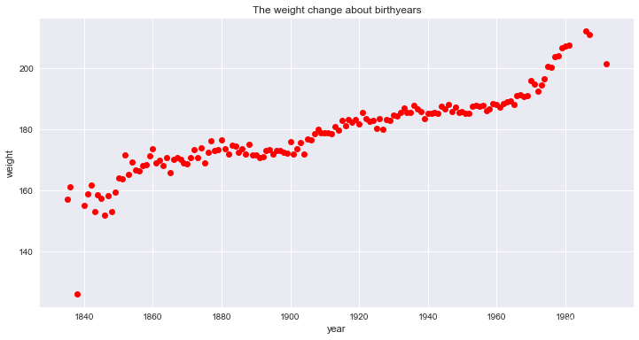
接下来,让我们看一下平均身高、平均体重岁随年份的变化
#提取数据
b=data1_df.groupby('birthYear').mean()

d=b.dropna()
#打印体重-时间折线图
print_plot(d,'weight','The weight change about birthyears')
<matplotlib.figure.Figure at 0xe404400>
#打印身高-时间折线图
print_plot(d,'height','The height change about birthYear')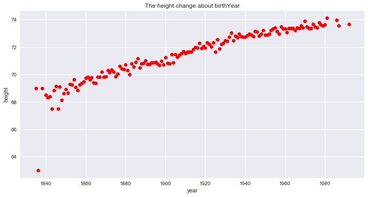
<matplotlib.figure.Figure at 0xe1509e8>
从这里可以看到,运动员的身高和体重随着出生年份呈现正相关关系。那么,他们之间有多大的相关性呢?接下来让我们查看一下
#提取数据
e=pd.DataFrame(d,columns=['birthyear','weight','height'])
e['birthyear']=e.index
#计算相关系数
e.corrwith(e['birthyear'])
birthyear 1.000000
weight 0.929546
height 0.947681
dtype: float64
从这里可以看到,运动员的出生年份与运动员的平均身高的的相关系数为0.947,与平均体重的相关系数为0.934。可以看到运动员的平均身高、体重与年份有很大的相关性。但是由于缺乏进一步数据,造成这种现象的原因不得而知
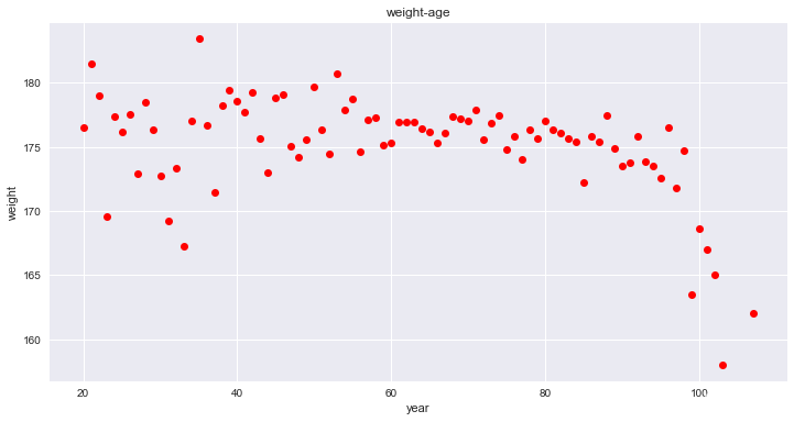
接下来,我们看一下运动员的寿命与身高、体重情况
#剔除在世运动员的数据,并提取数据
data_age=data1_df.dropna(how='all')
data_age=data_age[['playerID','birthYear','deathYear','weight','height']]
#计算运动员寿命
data_age=pd.DataFrame(data_age,columns=['playerID','birthYear','deathYear','Age','weight','height'])
data_age['Age']=data_age['deathYear']-data_age['birthYear']
去掉可能存在的缺失值
#剔除存在缺失的数据
data_age=data_age.dropna()
#计算平均值
f=data_age.groupby('Age').mean()
f| birthYear | deathYear | weight | height | |
|---|---|---|---|---|
| Age | ||||
| 20.0 | 1907.500000 | 1927.500000 | 176.500000 | 70.500000 |
| 21.0 | 1867.000000 | 1888.000000 | 181.500000 | 72.500000 |
| 22.0 | 1925.800000 | 1947.800000 | 179.000000 | 71.400000 |
| 23.0 | 1915.000000 | 1938.000000 | 169.600000 | 72.000000 |
| 24.0 | 1916.200000 | 1940.200000 | 177.400000 | 71.300000 |
| 25.0 | 1898.307692 | 1923.307692 | 176.153846 | 72.461538 |
| 26.0 | 1903.400000 | 1929.400000 | 177.533333 | 71.733333 |
| 27.0 | 1887.769231 | 1914.769231 | 172.884615 | 70.884615 |
| 28.0 | 1894.500000 | 1922.500000 | 178.500000 | 71.500000 |
| 29.0 | 1907.432432 | 1936.432432 | 176.297297 | 71.486486 |
| 30.0 | 1888.709677 | 1918.709677 | 172.774194 | 71.064516 |
| 31.0 | 1881.666667 | 1912.666667 | 169.259259 | 70.777778 |
| 32.0 | 1889.393939 | 1921.393939 | 173.333333 | 70.727273 |
| 33.0 | 1894.258065 | 1927.258065 | 167.290323 | 70.516129 |
| 34.0 | 1898.900000 | 1932.900000 | 177.040000 | 71.820000 |
| 35.0 | 1899.135135 | 1934.135135 | 183.405405 | 71.756757 |
| 36.0 | 1891.051282 | 1927.051282 | 176.717949 | 70.128205 |
| 37.0 | 1886.538462 | 1923.538462 | 171.461538 | 70.333333 |
| 38.0 | 1892.083333 | 1930.083333 | 178.250000 | 71.354167 |
| 39.0 | 1897.589744 | 1936.589744 | 179.435897 | 71.641026 |
| 40.0 | 1892.311111 | 1932.311111 | 178.555556 | 71.133333 |
| 41.0 | 1893.500000 | 1934.500000 | 177.704545 | 70.727273 |
| 42.0 | 1893.225000 | 1935.225000 | 179.225000 | 71.275000 |
| 43.0 | 1891.204082 | 1934.204082 | 175.673469 | 70.816327 |
| 44.0 | 1885.344262 | 1929.344262 | 173.016393 | 70.377049 |
| 45.0 | 1898.121212 | 1943.121212 | 178.848485 | 71.136364 |
| 46.0 | 1893.938776 | 1939.938776 | 179.040816 | 71.061224 |
| 47.0 | 1893.441558 | 1940.441558 | 175.012987 | 70.805195 |
| 48.0 | 1894.000000 | 1942.000000 | 174.164557 | 70.949367 |
| 49.0 | 1894.213115 | 1943.213115 | 175.590164 | 70.868852 |
| ... | ... | ... | ... | ... |
| 75.0 | 1900.285024 | 1975.285024 | 174.782609 | 71.164251 |
| 76.0 | 1897.894977 | 1973.894977 | 175.808219 | 71.118721 |
| 77.0 | 1897.607143 | 1974.607143 | 173.991071 | 71.004464 |
| 78.0 | 1897.606635 | 1975.606635 | 176.327014 | 71.033175 |
| 79.0 | 1898.990991 | 1977.990991 | 175.644144 | 71.157658 |
| 80.0 | 1899.351240 | 1979.351240 | 177.000000 | 71.190083 |
| 81.0 | 1899.879630 | 1980.879630 | 176.351852 | 70.925926 |
| 82.0 | 1900.754464 | 1982.754464 | 176.075893 | 71.281250 |
| 83.0 | 1901.454128 | 1984.454128 | 175.665138 | 71.243119 |
| 84.0 | 1898.257895 | 1982.257895 | 175.415789 | 70.915789 |
| 85.0 | 1900.005263 | 1985.005263 | 172.215789 | 70.968421 |
| 86.0 | 1903.913978 | 1989.913978 | 175.811828 | 71.209677 |
| 87.0 | 1897.798611 | 1984.798611 | 175.402778 | 71.090278 |
| 88.0 | 1904.540541 | 1992.540541 | 177.425676 | 71.533784 |
| 89.0 | 1900.299213 | 1989.299213 | 174.866142 | 71.228346 |
| 90.0 | 1901.486726 | 1991.486726 | 173.495575 | 70.858407 |
| 91.0 | 1899.068182 | 1990.068182 | 173.750000 | 70.681818 |
| 92.0 | 1901.673684 | 1993.673684 | 175.831579 | 71.157895 |
| 93.0 | 1901.513158 | 1994.513158 | 173.828947 | 71.000000 |
| 94.0 | 1898.088889 | 1992.088889 | 173.533333 | 71.311111 |
| 95.0 | 1899.461538 | 1994.461538 | 172.576923 | 70.826923 |
| 96.0 | 1902.222222 | 1998.222222 | 176.500000 | 71.111111 |
| 97.0 | 1893.647059 | 1990.647059 | 171.823529 | 70.352941 |
| 98.0 | 1900.882353 | 1998.882353 | 174.705882 | 70.705882 |
| 99.0 | 1897.222222 | 1996.222222 | 163.444444 | 69.666667 |
| 100.0 | 1899.700000 | 1999.700000 | 168.600000 | 70.100000 |
| 101.0 | 1900.400000 | 2001.400000 | 167.000000 | 70.400000 |
| 102.0 | 1900.000000 | 2002.000000 | 165.000000 | 71.000000 |
| 103.0 | 1911.000000 | 2014.000000 | 158.000000 | 65.000000 |
| 107.0 | 1891.000000 | 1998.000000 | 162.000000 | 69.000000 |
85 rows × 4 columns
#提取年龄
age_df=pd.DataFrame(f,columns=['age','weight','height'])
age_df['age']=f.index
#绘制折线图
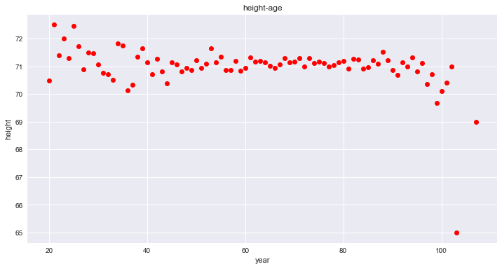
print_plot(age_df,'weight','weight-age')
print_plot(age_df,'height','height-age')
<matplotlib.figure.Figure at 0xe81df98>
<matplotlib.figure.Figure at 0xdfd5c50>
#计算相关系数
age_df.corr()| age | weight | height | |
|---|---|---|---|
| age | 1.000000 | -0.430298 | -0.371683 |
| weight | -0.430298 | 1.000000 | 0.724237 |
| height | -0.371683 | 0.724237 | 1.000000 |
可以看到,运动员寿命与身高、体重存在弱相关关系,且与运动员身高、体重呈负相关关系。其相关性远不如出生年份。但这里也说明运动员的身高、体重在某种程度上有可能影响运动员寿命


 6146
6146

 被折叠的 条评论
为什么被折叠?
被折叠的 条评论
为什么被折叠?
 到【灌水乐园】发言


