


因为KCF算法和CSK基本一样,因此关于KCF的笔记仅记录从section 4 开始的公式推导和理解。
为了表述清楚,本文所有小写加粗符号表示列向量,小写不加粗表示元素或参量,大写符号表示矩阵。
4 Building blocks
4.1 Linear regression
通过岭回归(ridge regression)或支持向量机(SVM)
min
w
∑
i
n
(
f
(
x
i
)
−
y
i
)
2
+
λ
∥
w
∥
2
\min_{\mathbf{w}}\sum_{i}^{n}(f(\mathbf{x}_{i})-y_{i})^2+\lambda\| \mathbf{w} \|^2
wmini∑n(f(xi)−yi)2+λ∥w∥2
分类器
f
(
x
i
)
=
w
T
x
i
f(\mathbf{x}_{i})=\mathbf{w}^T\mathbf{x}_{i}
f(xi)=wTxi
所以上式
=
min
w
∑
i
n
(
w
T
x
i
−
y
i
)
2
+
λ
∥
w
∥
2
=
min
w
∥
X
w
−
y
∥
2
+
λ
∥
w
∥
2
=
(
X
w
−
y
)
T
(
X
w
−
y
)
+
λ
w
T
w
\begin{aligned} &=\min_{\mathbf{w}}\sum_{i}^{n}(\mathbf{w}^T\mathbf{x}_{i}-y_{i})^2+\lambda\| \mathbf{w} \|^2\\ &=\min_{\mathbf{w}}\|X\mathbf{w}-\mathbf{y}\|^2+\lambda\| \mathbf{w} \|^2\\ &=(X\mathbf{w}-\mathbf{y})^T(X\mathbf{w}-\mathbf{y})+\lambda\mathbf{w}^T\mathbf{w}\\ \end{aligned}
=wmini∑n(wTxi−yi)2+λ∥w∥2=wmin∥Xw−y∥2+λ∥w∥2=(Xw−y)T(Xw−y)+λwTw
接下来是矩阵的求导,这里是分子布局(numerater layout)的标量/向量情况
∂
[
.
.
.
]
∂
w
=
2
(
X
w
−
y
)
T
∂
∂
w
(
X
w
−
y
)
+
2
λ
w
T
=
2
(
X
w
−
y
)
T
∂
∂
w
(
X
w
)
+
2
λ
w
T
=
2
(
X
w
−
y
)
T
X
+
2
λ
w
T
\begin{aligned} \frac{\partial[...] }{\partial \mathbf{w}} &=2(X\mathbf{w}-\mathbf{y})^T \frac{\partial}{\partial \mathbf{w}}(X\mathbf{w}-\mathbf{y}) +2\lambda \mathbf{w}^T\\ &=2(X\mathbf{w}-\mathbf{y})^T \frac{\partial}{\partial \mathbf{w}}(X\mathbf{w}) +2\lambda \mathbf{w}^T\\ &=2(X\mathbf{w}-\mathbf{y})^T X +2\lambda \mathbf{w}^T \end{aligned}
∂w∂[...]=2(Xw−y)T∂w∂(Xw−y)+2λwT=2(Xw−y)T∂w∂(Xw)+2λwT=2(Xw−y)TX+2λwT
令
∂
[
.
.
.
]
∂
w
=
0
\frac{\partial[...] }{\partial \mathbf{w}}=0
∂w∂[...]=0,有
w
T
X
T
X
−
y
T
X
+
λ
w
T
=
0
w
T
(
X
T
X
+
λ
I
)
=
y
T
X
w
T
=
(
X
X
T
+
λ
I
)
−
1
y
T
X
w
=
(
X
X
T
+
λ
I
)
−
1
X
T
y
\begin{aligned} \mathbf{w}^TX^TX-\mathbf{y}^TX+\lambda \mathbf{w}^T=0\\ \mathbf{w}^T(X^TX+\lambda I)=\mathbf{y}^TX\\ \mathbf{w}^T=(XX^T+\lambda I)^{-1}\mathbf{y}^TX\\ \mathbf{w}=(XX^T+\lambda I)^{-1}X^T\mathbf{y} \end{aligned}
wTXTX−yTX+λwT=0wT(XTX+λI)=yTXwT=(XXT+λI)−1yTXw=(XXT+λI)−1XTy
因为后续会变换到傅里叶域,所以将
X
T
X^T
XT处理为
(
X
∗
)
T
(X^*)^T
(X∗)T,记为
X
H
X^H
XH,所以
w
=
(
X
X
H
+
λ
I
)
−
1
X
H
y
\mathbf{w}=(XX^H+\lambda I)^{-1}X^H\mathbf{y}
w=(XXH+λI)−1XHy
4.2 Cyclic shift 4.3 Circulant matrics
引入循环矩阵增加样本量,首先讨论一维样本
x
\mathbf{x}
x的情况(n*1)
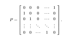
P
x
=
[
x
n
x
1
x
2
.
.
.
.
.
.
x
n
−
1
]
T
P\mathbf{x}=[x_{n}x_{1} x_{2}......x_{n-1}]^T
Px=[xnx1x2......xn−1]T
{
P
u
x
∣
u
=
0
,
1
,
2
,
.
.
.
,
n
}
\begin{Bmatrix} {P^u\mathbf{x}|u=0,1,2,...,n} \end{Bmatrix}
{Pux∣u=0,1,2,...,n}
u<[n/2]往正方向移动,u>[n/2]往相反方向移动,u>n循环为i=1的情况。
其循环位移的结果可以由图片简式
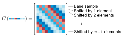
每一行都是上一行通过位移矩阵P位移一个元素的结果。
X
=
C
(
x
)
=
[
(
p
0
x
)
T
(
p
1
x
)
T
(
p
2
x
)
T
⋮
(
p
n
x
)
T
]
=
[
p
0
x
p
1
x
p
2
x
p
0
x
⋯
p
n
x
]
T
X=C(\mathbf{x})=\begin{bmatrix} (p^0\mathbf{x})^T\\ (p^1\mathbf{x})^T\\ (p^2\mathbf{x})^T\\ \vdots \\ (p^n\mathbf{x})^T \end{bmatrix} =\begin{bmatrix} p^0\mathbf{x}&p^1\mathbf{x}&p^2\mathbf{x}&p^0\mathbf{x}&\cdots &p^n\mathbf{x} \end{bmatrix}^T
X=C(x)=⎣⎢⎢⎢⎢⎢⎡(p0x)T(p1x)T(p2x)T⋮(pnx)T⎦⎥⎥⎥⎥⎥⎤=[p0xp1xp2xp0x⋯pnx]T
顺便一提,一维样本通过循环位移形成二维的循环矩阵,二维样本通过循环位移成为四维的循环矩阵(可以形象地理解为二维图片的处理有两个自由度(上下方向、左右方向),处理后的许多样本图片再堆叠起来)。
引入循环矩阵是将原来
x
i
\mathbf{x_{i}}
xi样本扩充为
C
(
x
i
)
C(\mathbf{x_{i}})
C(xi),增加样本数,提高准确率,但这样计算量不是大大增加吗,为什么还能简化运算?
之所以引入循环矩阵,还是为了利用循环矩阵的傅里叶对角化特性,将其转入傅里叶域加快计算。(其他特性及证明这里不多赘述)
(
1
)
X
=
C
(
x
)
=
F
⋅
d
i
a
g
(
x
^
)
⋅
F
H
(1)X=C(\mathbf{x})=F\cdot diag(\mathbf{\hat{x}})\cdot F^H
(1)X=C(x)=F⋅diag(x^)⋅FH
d
i
a
g
diag
diag是保留对角化元素形成矩阵(这里是矩阵,不是向量);相对文章简化一下,令
F
⋅
x
=
x
^
F\cdot \mathbf{x}=\mathbf{\hat{x}}
F⋅x=x^ ;
F
F
H
=
F
H
F
=
I
FF^H=F^HF=I
FFH=FHF=I
( 2 ) C ( x ) y = F − 1 ( F ∗ ( x ) ⋅ F ( y ) ) (2)C(\mathbf{x})\mathbf{y}=F^{-1}(F^*(\mathbf{x})\cdot F(\mathbf{y})) (2)C(x)y=F−1(F∗(x)⋅F(y))这个性质实质上是由上个式子推导得到。
4.4 Putting it all together
X
=
F
⋅
d
i
a
g
(
x
^
)
⋅
F
H
X=F\cdot diag(\mathbf{\hat{x}})\cdot F^H
X=F⋅diag(x^)⋅FH
X
H
=
(
F
H
)
H
⋅
d
i
a
g
(
x
^
∗
)
⋅
F
H
=
F
⋅
d
i
a
g
(
x
^
∗
)
⋅
F
H
X^H=(F^H)^H\cdot diag(\mathbf{\hat{x}}^*)\cdot F^H=F\cdot diag(\mathbf{\hat{x}}^*)\cdot F^H
XH=(FH)H⋅diag(x^∗)⋅FH=F⋅diag(x^∗)⋅FH
X
H
X
=
F
⋅
d
i
a
g
(
x
^
∗
)
⋅
(
F
H
⋅
F
)
⋅
d
i
a
g
(
x
^
)
⋅
F
H
=
F
⋅
d
i
a
g
(
x
^
∗
)
⋅
d
i
a
g
(
x
^
)
⋅
F
H
=
F
⋅
d
i
a
g
(
x
^
∗
⊙
x
^
)
⋅
F
H
\begin{aligned} X^HX&=F\cdot diag(\mathbf{\hat{x}}^*)\cdot (F^H\cdot F)\cdot diag(\mathbf{\hat{x}})\cdot F^H\\ &=F\cdot diag(\mathbf{\hat{x}}^*)\cdot diag(\mathbf{\hat{x}})\cdot F^H\\ &=F\cdot diag(\mathbf{\hat{x}}^*\odot \mathbf{\hat{x}})\cdot F^H\end{aligned}
XHX=F⋅diag(x^∗)⋅(FH⋅F)⋅diag(x^)⋅FH=F⋅diag(x^∗)⋅diag(x^)⋅FH=F⋅diag(x^∗⊙x^)⋅FH
设
I
=
C
(
δ
)
,
δ
=
[
1
0
0
.
.
.
0
]
T
,
δ
^
=
1
I=C\left ( \delta \right ),\delta=\begin{bmatrix} 1 & 0 & 0 &... & 0 \end{bmatrix}^T,\hat{\delta}=1
I=C(δ),δ=[100...0]T,δ^=1
C
(
δ
)
=
F
⋅
d
i
a
g
(
δ
^
)
⋅
F
H
=
F
I
F
H
C(\delta)=F\cdot diag(\hat{\delta})\cdot F^H=FIF^H
C(δ)=F⋅diag(δ^)⋅FH=FIFH
w
=
(
X
X
H
+
λ
I
)
−
1
X
H
y
=
(
X
H
X
+
λ
C
(
δ
)
)
−
1
X
H
y
=
(
F
⋅
d
i
a
g
(
x
^
∗
⊙
x
^
)
⋅
F
H
+
λ
F
I
F
H
)
−
1
X
H
y
=
(
F
d
i
a
g
(
x
^
∗
⊙
x
^
+
λ
)
F
H
)
−
1
X
H
y
=
(
F
d
i
a
g
(
x
^
∗
⊙
x
^
+
λ
)
−
1
F
H
)
X
H
y
=
F
d
i
a
g
(
x
^
∗
⊙
x
^
+
λ
)
−
1
(
F
H
F
)
d
i
a
g
(
x
^
∗
)
F
H
y
=
F
d
i
a
g
(
x
^
∗
x
^
∗
⊙
x
^
+
λ
)
F
H
y
=
C
(
F
−
1
(
x
^
∗
x
^
∗
⊙
x
^
+
λ
)
)
y
=
F
−
1
(
F
∗
(
F
−
1
(
x
^
∗
x
^
∗
⊙
x
^
+
λ
)
)
⊙
F
(
y
)
)
=
x
^
x
^
⊙
x
^
∗
+
λ
⊙
F
(
y
)
=
x
^
⊙
y
^
x
^
⊙
x
^
∗
+
λ
\begin{aligned} \mathbf{w}&=(XX^H+\lambda I)^{-1}X^H\mathbf{y}\\ &=(X^HX+\lambda C(\delta))^{-1}X^H\mathbf{y}\\ &=(F\cdot diag(\mathbf{\hat{x}}^*\odot \mathbf{\hat{x}})\cdot F^H+\lambda FIF^H)^{-1}X^H\mathbf{y}\\ &=(Fdiag(\mathbf{\hat{x}}^*\odot \mathbf{\hat{x}}+\lambda)F^H)^{-1}X^H\mathbf{y}\\ &=(Fdiag(\mathbf{\hat{x}}^*\odot \mathbf{\hat{x}}+\lambda)^{-1}F^H)X^H\mathbf{y}\\ &=Fdiag(\mathbf{\hat{x}}^*\odot \mathbf{\hat{x}}+\lambda)^{-1}(F^HF) diag(\mathbf{\hat{x}}^*)F^H\mathbf{y}\\ &=Fdiag(\frac{\mathbf{\hat{x}}^*}{\mathbf{\hat{x}}^*\odot \mathbf{\hat{x}}+\lambda})F^H\mathbf{y}\\\\ &=C(F^{-1}(\frac{\mathbf{\hat{x}}^*}{\mathbf{\hat{x}}^*\odot \mathbf{\hat{x}}+\lambda}))\mathbf{y}\\\\ &=F^{-1}(F^*(F^{-1}(\frac{\mathbf{\hat{x}}^*}{\mathbf{\hat{x}}^*\odot \mathbf{\hat{x}}+\lambda}))\odot F(\mathbf{y}))\\\\ &=\frac{\mathbf{\hat{x}}}{\mathbf{\hat{x}}\odot \mathbf{\hat{x}}^*+\lambda}\odot F(\mathbf{y})\\\\ &=\frac{\mathbf{\hat{x}}\odot\mathbf{\hat{y}}}{\mathbf{\hat{x}}\odot \mathbf{\hat{x}}^*+\lambda} \end{aligned}
w=(XXH+λI)−1XHy=(XHX+λC(δ))−1XHy=(F⋅diag(x^∗⊙x^)⋅FH+λFIFH)−1XHy=(Fdiag(x^∗⊙x^+λ)FH)−1XHy=(Fdiag(x^∗⊙x^+λ)−1FH)XHy=Fdiag(x^∗⊙x^+λ)−1(FHF)diag(x^∗)FHy=Fdiag(x^∗⊙x^+λx^∗)FHy=C(F−1(x^∗⊙x^+λx^∗))y=F−1(F∗(F−1(x^∗⊙x^+λx^∗))⊙F(y))=x^⊙x^∗+λx^⊙F(y)=x^⊙x^∗+λx^⊙y^
4.5 relationship to correlation filter
之前已经总结过,这里不赘述。
相关滤波跟踪·MOSSE算法的梳理
相关滤波跟踪·CSK算法梳理(巨详(啰)细(嗦))
5. Non-linear regression
5.1 kernel trick - brief overview
第四部分讨论的是样本线性可分的情况的,当样本线性不可分时,将样本映射到高维空间使线性可分。
但不仅这个映射关系复杂无规律,而且在高维空间的点乘计算量巨大,易产生“维数灾难”,所以利用核函数技巧(kernel trick),通过一些特殊的核函数将高维空间的运算等同到低维空间来。
这部分具体解释见SVM学习整理·结合CSK\KCF
映射关系
x
i
→
φ
(
x
i
)
\mathbf{x}_{i}\rightarrow \varphi (\mathbf{x}_{i})
xi→φ(xi)
分类器权重
w
\mathbf{w}
w的线性组合
w
=
∑
j
n
α
j
φ
(
x
j
)
\mathbf{w}=\sum_{j}^{n}\alpha_{j}\varphi (\mathbf{x}_{j})
w=∑jnαjφ(xj)
岭回归表示为
min
∑
i
(
f
(
φ
(
x
i
)
)
−
y
i
)
2
+
λ
∥
w
∥
2
=
min
∑
i
(
∑
j
α
j
φ
T
(
x
j
)
φ
(
x
i
)
−
y
i
)
2
+
λ
∥
w
∥
2
=
min
(
φ
T
(
X
)
φ
(
X
)
α
−
y
i
)
2
+
λ
α
T
φ
T
(
X
)
φ
(
X
)
α
\begin{aligned} &\min\sum_{i}(f(\varphi(\mathbf{x}_{i}))-y_{i})^2+\lambda\|\mathbf{w}\|^2\\ =&\min\sum_{i}(\sum_{j}\alpha_{j}\varphi^T(\mathbf{x}_{j})\varphi(\mathbf{x}_{i})-y_{i})^2+\lambda\|\mathbf{w}\|^2\\ =&\min(\varphi^T(X)\varphi(X)\boldsymbol{\alpha}-\mathbf{y}_{i})^2+\lambda\boldsymbol{\alpha}^T\varphi^T(X)\varphi(X)\boldsymbol{\alpha}\\ \end{aligned}
==mini∑(f(φ(xi))−yi)2+λ∥w∥2mini∑(j∑αjφT(xj)φ(xi)−yi)2+λ∥w∥2min(φT(X)φ(X)α−yi)2+λαTφT(X)φ(X)α
(
h
e
r
e
,
X
i
j
=
x
i
T
x
j
)
(here, X_{ij}=\mathbf{x}_{i}^T\mathbf{x}_{j})
(here,Xij=xiTxj)
令
K
=
φ
T
(
X
)
φ
(
X
)
K
i
j
=
φ
T
(
x
i
)
φ
(
x
j
)
=
κ
(
x
i
,
x
j
)
\begin{aligned}&K=\varphi^T(X)\varphi(X)\\ &K_{ij}=\varphi^T(\mathbf{x}_{i})\varphi(\mathbf{x}_{j})=\kappa (\mathbf{x}_{i},\mathbf{x}_{j})\end{aligned}
K=φT(X)φ(X)Kij=φT(xi)φ(xj)=κ(xi,xj)
5.2 fast kernel regression
现引入循环操作矩阵
P
P
P(此处有附录A.2证明
K
K
K可以随
X
X
X是循环矩阵而是循环矩阵的证明过程:
X
X
X是(j-i)%n的循环,
K
K
K也是(j-i)%n的循环)
x
i
=
P
i
x
x
j
=
P
j
x
K
i
j
=
φ
T
(
P
i
x
)
φ
(
P
j
x
)
=
κ
(
P
i
x
,
P
j
x
)
=
κ
(
p
−
i
P
i
x
,
p
−
i
P
j
x
)
=
κ
(
x
,
P
j
−
i
x
)
\begin{aligned} &\mathbf{x}_{i}=P^i\mathbf{x}\\ &\mathbf{x}_{j}=P^j\mathbf{x}\\ &K_{ij}=\varphi^T(P^i\mathbf{x})\varphi(P^j\mathbf{x})=\kappa (P^i\mathbf{x},P^j\mathbf{x})=\kappa (p^{-i}P^i\mathbf{x},p^{-i}P^j\mathbf{x})=\kappa (\mathbf{x},P^{j-i}\mathbf{x})\end{aligned}
xi=Pixxj=PjxKij=φT(Pix)φ(Pjx)=κ(Pix,Pjx)=κ(p−iPix,p−iPjx)=κ(x,Pj−ix)(此处利用了文中定理1)
现在,已知
K
K
K是循环矩阵,那么求他的生成向量,也就是求这个矩阵的第一行。
即,令
i
=
1
i=1
i=1,
K
1
j
=
=
κ
(
x
,
P
j
−
1
x
)
K_{1j}==\kappa (\mathbf{x},P^{j-1}\mathbf{x})
K1j==κ(x,Pj−1x),也表示为
k
i
x
x
=
φ
T
(
x
)
φ
(
P
i
−
1
x
)
=
κ
(
x
,
P
i
−
1
x
)
\mathbf{k}_{i}^{\mathbf{xx}}=\varphi^T(\mathbf{x})\varphi(P^{i-1}\mathbf{x})=\kappa(\mathbf{x},P^{i-1}\mathbf{x})
kixx=φT(x)φ(Pi−1x)=κ(x,Pi−1x)
回到求解滤波器上,即求解
α
\alpha
α
α
=
(
K
+
λ
I
)
−
1
y
=
(
C
(
k
x
x
)
+
λ
I
)
−
1
y
=
(
F
d
i
a
g
(
k
^
x
x
)
F
H
+
λ
F
d
i
a
g
(
δ
^
)
F
H
)
−
1
y
=
(
F
d
i
a
g
(
k
^
x
x
+
λ
)
−
1
F
H
)
y
\begin{aligned} \boldsymbol{\alpha}=&(K+\lambda I)^{-1}\mathbf{y}\\ &=(C(\mathbf{k^{xx}})+\lambda I)^{-1}\mathbf{y}\\ &=(Fdiag(\mathbf{\hat{k}^{xx}})F^H+\lambda Fdiag(\hat{\delta})F^H)^{-1}\mathbf{y}\\ &=(Fdiag(\mathbf{\hat{k}^{xx}}+\lambda)^{-1}F^H)\mathbf{y}\\ \end{aligned}
α=(K+λI)−1y=(C(kxx)+λI)−1y=(Fdiag(k^xx)FH+λFdiag(δ^)FH)−1y=(Fdiag(k^xx+λ)−1FH)y
两边同乘以
F
H
F^H
FH
F
H
α
=
d
i
a
g
(
k
^
x
x
+
λ
)
−
1
F
H
y
α
^
∗
=
d
i
a
g
(
1
k
^
x
x
+
λ
)
y
^
∗
=
y
^
∗
k
^
x
x
+
λ
\begin{aligned} F^H\boldsymbol{\alpha}&=diag(\mathbf{\hat{k}^{xx}}+\lambda)^{-1}F^H\mathbf{y}\\ \boldsymbol{\hat{\alpha}}^*&=diag(\frac{1}{\mathbf{\hat{k}^{xx}}+\lambda})\mathbf{\hat{y}}^*\\ &=\frac{\mathbf{\hat{y}}^*}{\mathbf{\hat{k}^{xx}}+\lambda} \end{aligned}
FHαα^∗=diag(k^xx+λ)−1FHy=diag(k^xx+λ1)y^∗=k^xx+λy^∗
5.3 fast detection
这部分只是把其中一个样本
x
\mathbf{x}
x换成在该帧中上一帧的位置取的图像
z
\mathbf{z}
z
y
^
=
f
^
(
z
)
=
k
^
x
z
α
^
\mathbf{\hat{y}}=\mathbf{\hat{f}(z)}=\mathbf{\hat{k}^{xz}}\boldsymbol{\hat{\alpha}}
y^=f^(z)=k^xzα^
6 fast kernel correlation
这部分讲了符合循环矩阵的几种核函数的具体形式
6.1 dot-product and polynomial kernels
6.2 Radial Basis Function and Guassian kernels
6.3 other kernels
eg:intersection kernel
KCF的公式推导笔记基本上就是这样,欢迎讨论。
[181118]
%这周先交差,第五部分第六部分明天再写
[181122]
%线性回归里的下标就是循环产生的虚拟样本


 3万+
3万+


 被折叠的 条评论
为什么被折叠?
被折叠的 条评论
为什么被折叠?
 到【灌水乐园】发言


