边缘检测基础

最新推荐文章于 2024-04-13 16:06:01 发布

凡尘code

最新推荐文章于 2024-04-13 16:06:01 发布

阅读量356

点赞数 1

分类专栏：算法笔记

本文链接：https://blog.csdn.net/qq_33466466/article/details/124993793

版权

算法同时被 2 个专栏收录

24 篇文章 1 订阅

订阅专栏

笔记

19 篇文章 0 订阅

订阅专栏

边缘检测

边缘检测的一般步骤

滤波

边缘检测的算法主要是基于图像强度的一阶和二阶导数，但导数通常对噪声很敏感，因此必须采用滤波器来改善与噪声有关的边缘检测器的性能，常见的滤波方法主要有高斯滤波，即采用离散化的高斯函数产生一组归一化的高斯核，然后基于高斯核函数对图像灰度矩阵的每一点进行加权求和
增强

增强边缘的基础是确定图像各点邻域强度的变化值。增强算法可以将图像灰度点邻域强度值有显著变化的点凸显出来，在具体编程实现时，可通过计算梯度幅值来确定
检测

经过增强的图像，往往邻域中有很多点的梯度值比较大，而在特定的应用中，这些点并不是要找的边缘点，所以应该采用某种方法来对这些点进行取舍。实际工程中，常用的方法是通过阈值化方法来检测的

Canny算子

Canny的目标是找到一个最优的边缘检测算法，最优边缘检测的三个主要评价标准：

低错误率：标识出尽可能多的实际边缘，同时尽可能减少噪声产生的误报
高定位性：标识出的边缘要与图像中的实际边缘尽可能接近
最小响应：图像中的边缘只能标识一次，并且可能存在的图像噪声不应该被标识为边缘

为满足这些要求，Canny使用变分法，这是一种寻找满足特定功能的函数方法。最优检测用4个指数函数项的和表示，但是它非常近似于高斯函数的一阶导数

Canny边缘检测的步骤

消除噪声

一般情况下，使用高斯平滑滤波器卷积降噪。以下显示一个 $s i z e = 5$ 的高斯内核示例:
$\dfrac{1}{139} \begin{bmatrix} 2 & 4 & 5 & 4 & 2 \\ 4 & 9 & 12 & 9 & 4 \\ 5 & 12 & 15 & 12 & 5 \\ 4 & 9 & 12 & 9 & 4 \\ 2 & 4 & 5 & 4 & 2 \end{bmatrix}$
计算梯度幅值和方向

此处，按照Sobel滤波器的步骤来操作
- 运用一对卷积阵列（分别作用于x和y方向）
  $G_{x} = \begin{bmatrix} -1 & 0 & +1 \\ -2 & 0 & +2 \\ -1 & 0 & +1 \end{bmatrix} \qquad G_{y} = \begin{bmatrix} -1 & -2 & -1 \\ 0 & 0 & 0 \\ +1 & +2 & +1 \end{bmatrix}$
- 使用下列公式计算梯度幅值和方向
  $\sqrt{G^{2}_{x} + G^{2}_{y}} \\ \varTheta = \arctan \begin{pmatrix} \dfrac{G_y}{G_x} \end{pmatrix}$
  而梯度方向一般取这四个可能的角度之一—— $0^{\circ}、45^{\circ}、90^{\circ}、135^{\circ}$
非极大值抑制

这一步排除非边缘像素，仅仅保留一些细线条（候选边缘）
滞后阈值

这是最后一步，Canny使用了滞后阈值，滞后阈值需要两个阈值（高阈值和低阈值）：
1. 若某一像素位置的幅值超过了高阈值，该像素将被保留为边缘像素
2. 若某一像素的幅值低于低阈值，该像素将被排除
3. 若某一像素位置的幅值在两个阈值之间，该像素仅仅在连接到一个高于高阈值的像素时被保留

Canny()函数

Canny函数使用Canny算子来进行图像的边缘检测操作，函数原型如下：


/** @brief Finds edges in an image using the Canny algorithm @cite Canny86 .

The function finds edges in the input image and marks them in the output map edges using the
Canny algorithm. The smallest value between threshold1 and threshold2 is used for edge linking. The
largest value is used to find initial segments of strong edges. See
<http://en.wikipedia.org/wiki/Canny_edge_detector>

@param image 8-bit input image.
@param edges output edge map; single channels 8-bit image, which has the same size as image .
@param threshold1 first threshold for the hysteresis procedure.
@param threshold2 second threshold for the hysteresis procedure.
@param apertureSize aperture size for the Sobel operator.
@param L2gradient a flag, indicating whether a more accurate \f$L_2\f$ norm
\f$=\sqrt{(dI/dx)^2 + (dI/dy)^2}\f$ should be used to calculate the image gradient magnitude (
L2gradient=true ), or whether the default \f$L_1\f$ norm \f$=|dI/dx|+|dI/dy|\f$ is enough (
L2gradient=false ).
 */
CV_EXPORTS_W void Canny( InputArray image, OutputArray edges,
                         double threshold1, double threshold2,
                         int apertureSize = 3, bool L2gradient = false );

参数详情：

image: InputArray类型的image，即输入图像（源图像），填Mat类型的参数即可，需要为单通道8位图像。
edges：OutputArray类型的edges，输出的边缘图像，需要与输入图像有一样的尺寸和类型
threshold1:第一个滞后阈值
threshold2：第二个滞后阈值
apertureSize：表示引用Sobel算子的孔径大小，有默认值3
L2gradient：计算图像梯度幅值的标识

函数中的高低阈值中较小的值用于边缘连接，较大的阈值用于控制强边缘的初始段，推荐的高低阈值比值在 $\sim 3:1$ 之间

使用示例：

// 加载原始图像
Mat src = imread("1.png");
Mat dst;
Canny(src,dst,3,9,3);
imshow("边缘检测",dst);
waitKey(0);

示例程序

#include <iostream>
#include <opencv2/opencv.hpp>
#include<opencv2/highgui/highgui.hpp>
#include<opencv2/imgproc/imgproc.hpp>
using namespace cv;


int main()
{
	//载入原始图  
	Mat srcImage = imread(R"(1.jpg)");
	//工程目录下应该有一张名为1.jpg的素材图
	Mat srcImage1 = srcImage.clone();

	//显示原始图 
	imshow("【原始图】Canny边缘检测", srcImage);

	//----------------------------------------------------------------------------------
	//	一、最简单的canny用法，拿到原图后直接用。
	//	注意：此方法在OpenCV2中可用，在OpenCV3中已失效
	//----------------------------------------------------------------------------------
	//Canny( srcImage, srcImage, 150, 100,3 );
	//imshow("【效果图】Canny边缘检测", srcImage);

	Mat dst;
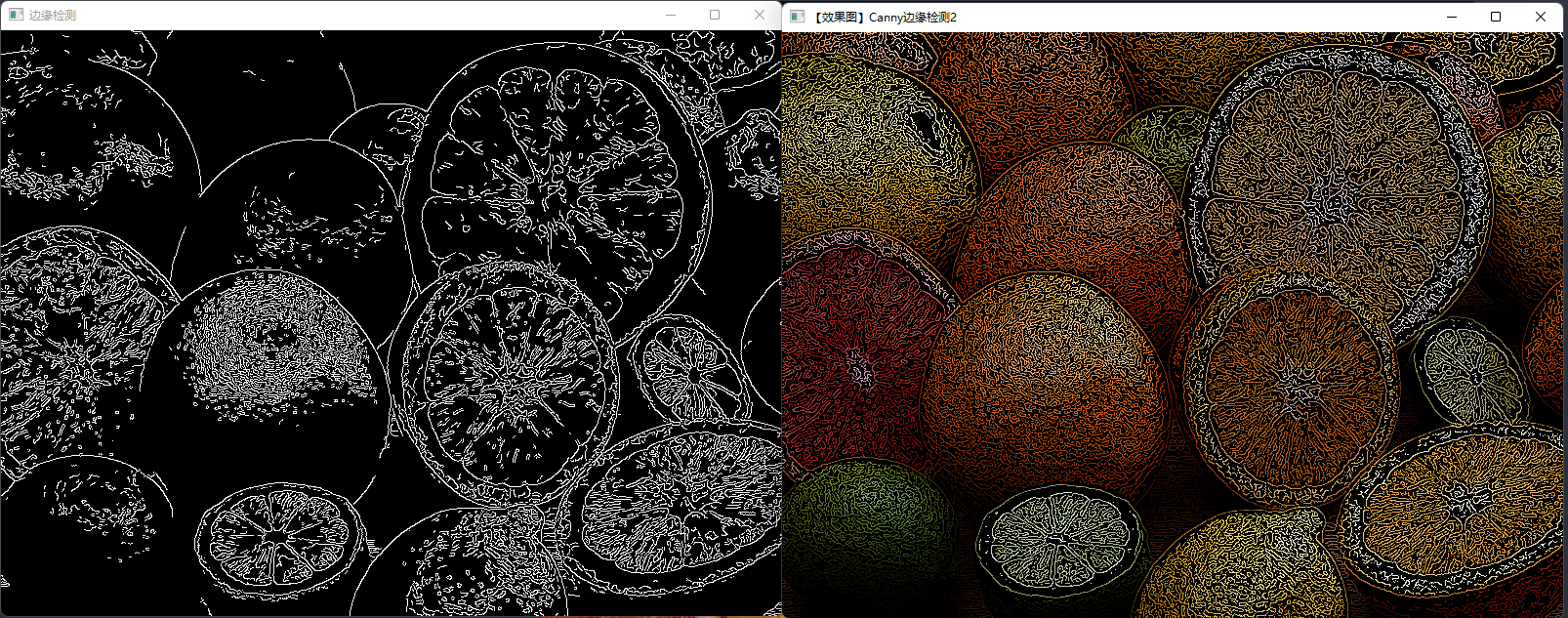
	Canny(srcImage, dst, 150, 100, 3);
	imshow("边缘检测", dst);


	//----------------------------------------------------------------------------------
	//	二、高阶的canny用法，转成灰度图，降噪，用canny，最后将得到的边缘作为掩码，拷贝原图到效果图上，得到彩色的边缘图
	//----------------------------------------------------------------------------------
	Mat dstImage, edge, grayImage;

	// 【1】创建与src同类型和大小的矩阵(dst)
	dstImage.create(srcImage1.size(), srcImage1.type());

	// 【2】将原图像转换为灰度图像
	cvtColor(srcImage1, grayImage, COLOR_BGR2GRAY);

	// 【3】先用使用 3x3内核来降噪
	blur(grayImage, edge, Size(3, 3));

	// 【4】运行Canny算子
	Canny(edge, edge, 3, 9, 3);

	//【5】将g_dstImage内的所有元素设置为0 
	dstImage = Scalar::all(0);

	//【6】使用Canny算子输出的边缘图g_cannyDetectedEdges作为掩码，来将原图g_srcImage拷到目标图g_dstImage中
	srcImage1.copyTo(dstImage, edge);

	//【7】显示效果图 
	imshow("【效果图】Canny边缘检测2", dstImage);


	waitKey(0);

	return 0;
}
// 代码来自：《OpenCV3编程入门》OpenCV3版书本配套示例程序56

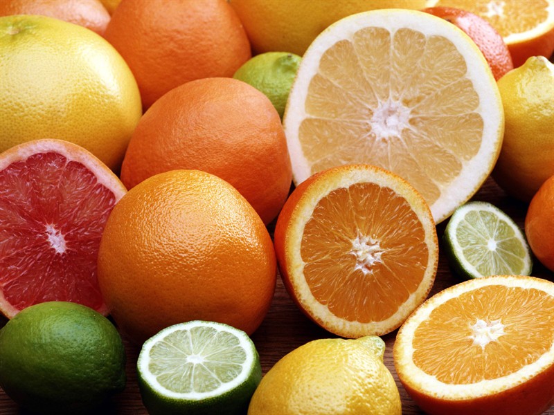
原始图片：

运行结果：

Sobel算子

Sobel算子是一个主要用于边缘检测的离散微分算子，结合了高斯平滑和微分求导，用来计算图像灰度函数的近似梯度，在图像的任何一点使用该算子，都将会产生对应的梯度矢量和其法矢量。

计算过程

在x和y两个方向上求导
1. 水平变化：将图像与一个奇数大小的内核 $G_{x}$ 进行卷积，比如：当内核大小为3时， $G_x$ 的计算结果为：
  $G_x = \begin{bmatrix} -1 & 0 & +1 \\ -2 & 0 & +2 \\ -1 & 0 & +1 \end{bmatrix} * I$
2. 垂直变化：将图像 $I$ 与一个奇数大小的内核进行卷积。比如当内核大小为3时，计算结果为：
  $G_y = \begin{bmatrix} -1 & -2 & +1 \\ 0 & 0 & 0 \\ +1 & +2 & +1 \end{bmatrix} * I$
在图像的每一点，结合以上两个结果求出近似梯度：
$\sqrt{G^{2}_{x} + G^{2}_{y}}$
另外有时，也可以使用下面更简单的公式代替：
$\left|G_x\right| + \left|G_y\right|$

Sobel()函数

Sobel()函数使用拓展的Sobel算子，来计算一阶、二阶、三阶或混合图像差分。

CV_EXPORTS_W void Sobel( 
    InputArray src, 
    OutputArray dst, 
    int ddepth,                
    int dx, 
    int dy, 
    int ksize = 3,
    double scale = 1, 
    double delta = 0,
    int borderType = BORDER_DEFAULT 
);

代码示例

#include <iostream>
#include <opencv2/opencv.hpp>
#include<opencv2/highgui/highgui.hpp>
#include<opencv2/imgproc/imgproc.hpp>
using namespace cv;


int main()
{
	//【0】创建 grad_x 和 grad_y 矩阵
	Mat grad_x, grad_y;
	Mat abs_grad_x, abs_grad_y, dst;

	//【1】载入原始图  
	Mat src = imread("1.jpg");  //工程目录下应该有一张名为1.jpg的素材图

	//【2】显示原始图 
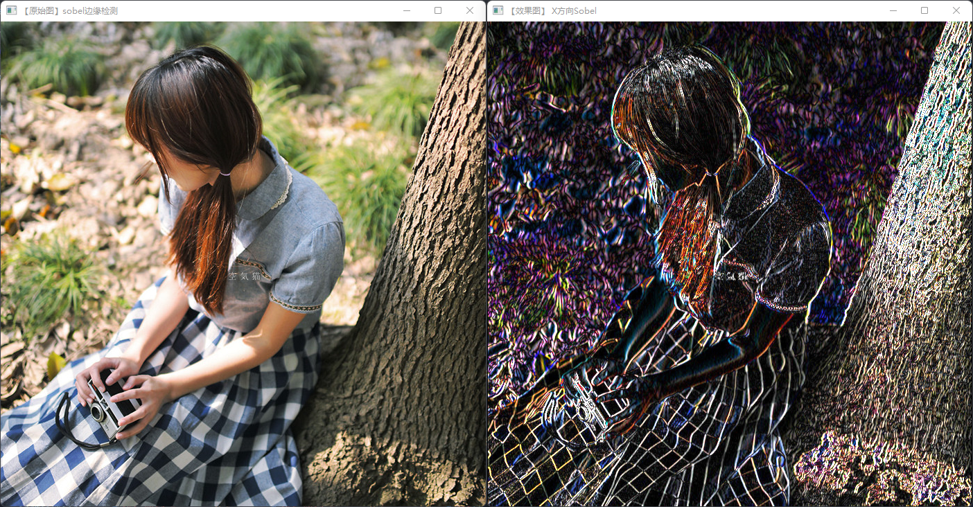
	imshow("【原始图】sobel边缘检测", src);

	//【3】求 X方向梯度
	Sobel(src, grad_x, CV_16S, 1, 0, 3, 1, 1, BORDER_DEFAULT);
	convertScaleAbs(grad_x, abs_grad_x);
	imshow("【效果图】 X方向Sobel", abs_grad_x);

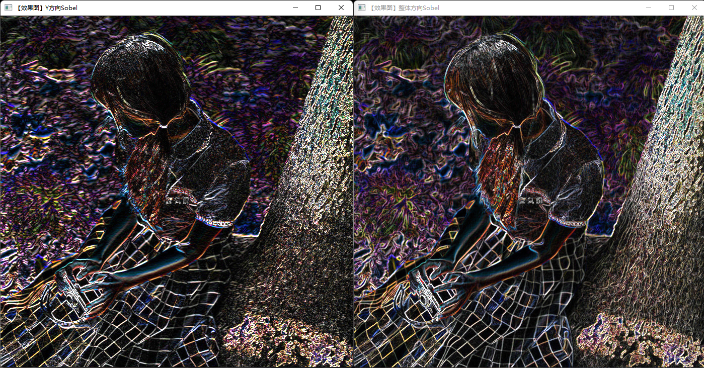
	//【4】求Y方向梯度
	Sobel(src, grad_y, CV_16S, 0, 1, 3, 1, 1, BORDER_DEFAULT);
	convertScaleAbs(grad_y, abs_grad_y);
	imshow("【效果图】Y方向Sobel", abs_grad_y);

	//【5】合并梯度(近似)
	addWeighted(abs_grad_x, 0.5, abs_grad_y, 0.5, 0, dst);
	imshow("【效果图】整体方向Sobel", dst);

	waitKey(0);
	return 0;
}

运行结果：

Laplacian算子

Laplacian算子是 $n$ 维欧几里得空间中的一个二阶微分算子，定义为梯度grad散度div 。因此如果 $f$ 是二阶可微的实函数，则 $f$ 的拉普拉斯算子定义如下：

$f$ 的拉普拉斯算子也是笛卡尔坐标系xi中的所有非混合二阶偏导数求和。

作为一个二阶微分算子，拉普拉斯算子把C函数映射到C函数。对于 $k\geq 2$ ，表达式（1）（或（2））定义了一个算子： $\Delta: C(R)\rightarrow C(R)$ ；或更一般地，对于任何开集 $\Omega$ ，定义一个算子 $\Delta: C(\Omega)\rightarrow C(\Omega)$

根据图像处理的原理可知，二阶导数可以用来进行边缘检测。因为图像是“二维”，需要在两个方向上进行求导。使用Laplacian算子将会使求导过程变得简单。

Laplacian算子的定义：
$\dfrac{\partial^{2}f}{\partial x^{2}} + \dfrac{\partial^{2}f}{\partial y^2}$
需要说明的是，由于Laplacian使用图像梯度，它内部的代码其实是调用了Sobel算子的。

让一幅图像减去它的Laplacian算子可以增强对比度。

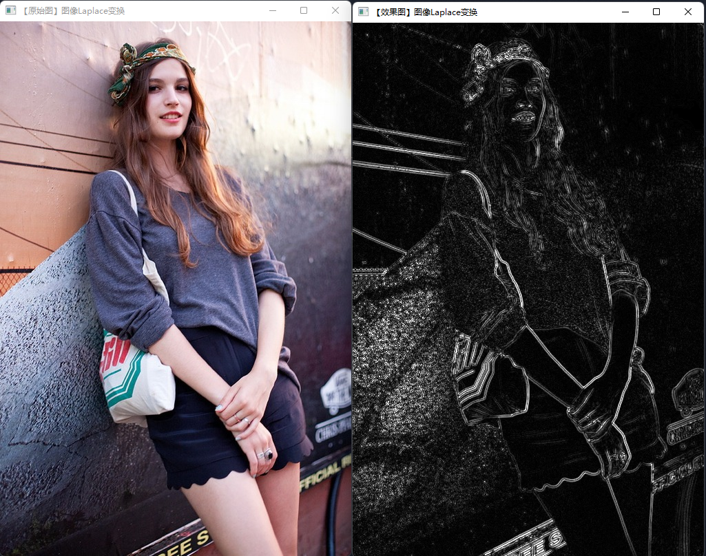
Laplacian算子使用

#include <iostream>
#include <opencv2/opencv.hpp>
#include<opencv2/highgui/highgui.hpp>
#include<opencv2/imgproc/imgproc.hpp>
using namespace cv;


int main()
{
	//【0】变量的定义
	Mat src, src_gray, dst, abs_dst;

	//【1】载入原始图  
	src = imread("E:\\git\\1.jpg");  //工程目录下应该有一张名为1.jpg的素材图

	//【2】显示原始图 
	imshow("【原始图】图像Laplace变换", src);

	//【3】使用高斯滤波消除噪声
	GaussianBlur(src, src, Size(3, 3), 0, 0, BORDER_DEFAULT);

	//【4】转换为灰度图
	cvtColor(src, src_gray, COLOR_RGB2GRAY);

	//【5】使用Laplace函数
	Laplacian(src_gray, dst, CV_16S, 3, 1, 0, BORDER_DEFAULT);

	//【6】计算绝对值，并将结果转换成8位
	convertScaleAbs(dst, abs_dst);

	//【7】显示效果图
	imshow("【效果图】图像Laplace变换", abs_dst);

	waitKey(0);
	return 0;
}

运行结果：

Scharr滤波器

使用示例：

//---------------------------------【头文件、命名空间包含部分】----------------------------
//		描述：包含程序所使用的头文件和命名空间
//------------------------------------------------------------------------------------------------
#include <opencv2/opencv.hpp>
#include<opencv2/highgui/highgui.hpp>
#include<opencv2/imgproc/imgproc.hpp>
using namespace cv;



//-----------------------------------【main( )函数】--------------------------------------------
//            描述：控制台应用程序的入口函数，我们的程序从这里开始
//-----------------------------------------------------------------------------------------------
int main( )
{
	//【0】创建 grad_x 和 grad_y 矩阵
	Mat grad_x, grad_y;
	Mat abs_grad_x, abs_grad_y,dst;

	//【1】载入原始图  
	Mat src = imread("1.jpg");  //工程目录下应该有一张名为1.jpg的素材图

	//【2】显示原始图 
	imshow("【原始图】Scharr滤波器", src); 

	//【3】求 X方向梯度
	Scharr( src, grad_x, CV_16S, 1, 0, 1, 0, BORDER_DEFAULT );
	convertScaleAbs( grad_x, abs_grad_x );
	imshow("【效果图】 X方向Scharr", abs_grad_x); 

	//【4】求Y方向梯度
	Scharr( src, grad_y, CV_16S, 0, 1, 1, 0, BORDER_DEFAULT );
	convertScaleAbs( grad_y, abs_grad_y );
	imshow("【效果图】Y方向Scharr", abs_grad_y); 

	//【5】合并梯度(近似)
	addWeighted( abs_grad_x, 0.5, abs_grad_y, 0.5, 0, dst );

	//【6】显示效果图
	imshow("【效果图】合并梯度后Scharr", dst); 

	waitKey(0); 
	return 0; 
}

原图：

运行结果：

凡尘code

关注

1
点赞
踩
1

收藏

觉得还不错? 一键收藏
0
评论
边缘检测基础

边缘检测边缘检测的一般步骤滤波边缘检测的算法主要是基于图像强度的一阶和二阶导数，但导数通常对噪声很敏感，因此必须采用滤波器来改善与噪声有关的边缘检测器的性能，常见的滤波方法主要有高斯滤波，即采用离散化的高斯函数产生一组归一化的高斯核，然后基于高斯核函数对图像灰度矩阵的每一点进行加权求和增强增强边缘的基础是确定图像各点邻域强度的变化值。增强算法可以将图像灰度点邻域强度值有显著变化的点凸显出来，在具体编程实现时，可通过计算梯度幅值来确定检测经过增强的图像，往往邻域中有很多点的梯度值比较
复制链接

扫一扫