机器学习(8)--创建KNN分类器

创建KNN分类器

KNN(k-nearest neighbors) 是使用k个最近邻的训练数据集来寻找对象分类的方法,如果希望将数据分类 可以找到一个KNN并做一个多数表决

代码实现如下:

# -*- coding:utf-8 -*-
# 导入基本模块
import numpy as np
import matplotlib.pyplot as plt
import matplotlib.cm as cm
from sklearn import neighbors,datasets

# 定义加载数据
def load_data(input_file):
    X = []
    with open(input_file, 'r') as f:
        for line in f.readlines():
            data = [float(x) for x in line.split(',')]
            X.append(data)
    return np.array(X)
# 加载输入数据
input_file = 'data_nn_classifier.txt'
data= load_data(input_file)

# 前两列代表输入数据 最后一列代表标签
x, y = data[:, :-1],data[:, -1].astype(np.int)

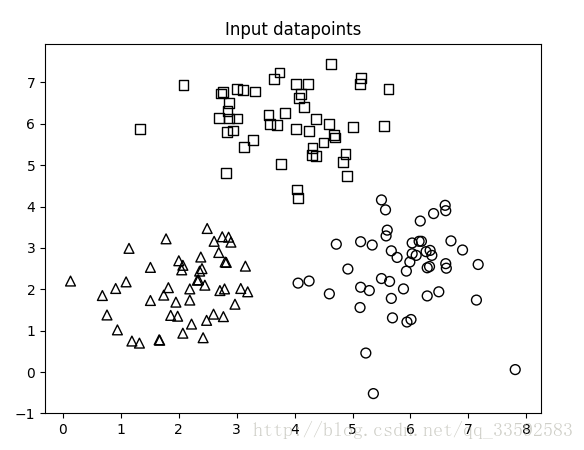
# 输入数据可视化
plt.figure()
plt.title('Input datapoints')
markers = '^sov<>hp'
mapper = np.array([markers[i] for i in y])

# x.shape[0] 表示行数,x.shape[1]代表列数
# 迭代所有数据点,并用合适的标记区分不同类
for i in range(x.shape[0]):
    plt.scatter(x[i,0],x[i,1],marker=mapper[i],s=50,edgecolors='black',facecolors='none')

# 构建分类器
# 设置最近邻的个数
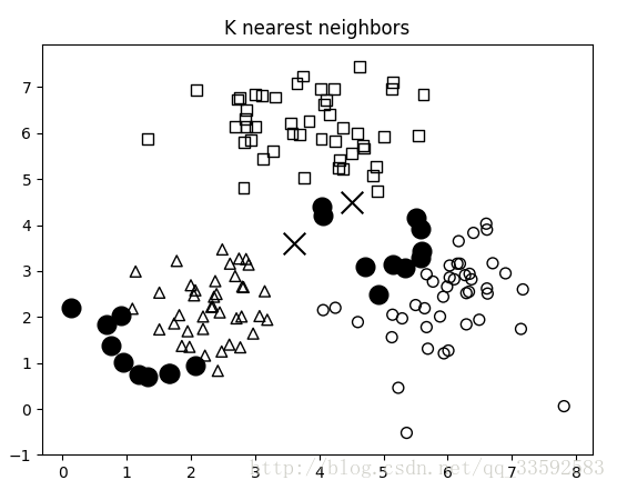
num_neighbors = 10

# 边界可视化 定义网格 用网格评价分类器
# 定义网格步长
h = 0.01

# 创建KNN分类器模型并进行训练

classifier = neighbors.KNeighborsClassifier(num_neighbors,weights='distance')
classifier.fit(x,y)

# 建立网格画出边界 对网格进行定义
# x坐标的第一列的最小值与最大值
x_min,x_max = x[:,0].min()-1,x[:,0].max()+1
y_min,y_max = x[:,1].min()-1,x[:,1].max()+1
x_grid,y_grid = np.meshgrid(np.arange(x_min,x_max,h),np.arange(y_min,y_max,h))

# 评价分类器对所有点的输出
predicted_values = classifier.predict(np.c_[x_grid.ravel(), y_grid.ravel()])

# 画出计算结果
predicted_values=predicted_values.reshape(x_grid.shape)
plt.figure()
plt.pcolormesh(x_grid,y_grid,predicted_values,cmap=cm.Pastel1)

# 在图中画出训练数据点
for i in range(x.shape[0]):
    plt.scatter(x[i,0],x[i,1],marker=mapper[i],s=50,edgecolors='black',facecolors='none')
plt.xlim(x_grid.min(),x_grid.max())
plt.ylim(y_grid.min(),y_grid.max())
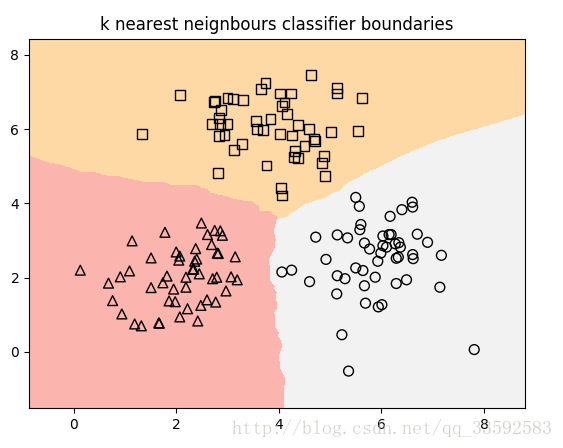
plt.title('k nearest neignbours classifier boundaries')

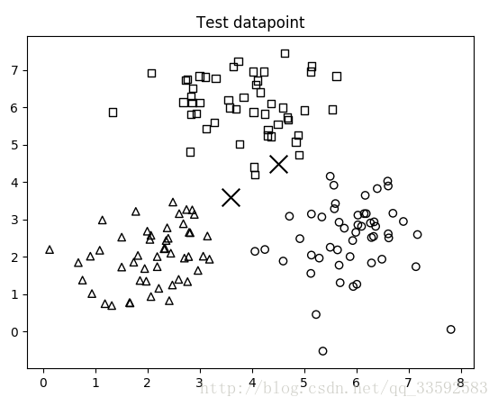
#  测试输入数据点
test_datapoint = [[4.5,3.6]]
plt.figure()
plt.title('Test datapoint')
for i in range(x.shape[0]):
  plt.scatter(x[i,0],x[i,1],marker=mapper[i],edgecolors='black',facecolors='none')
plt.scatter(test_datapoint[0],test_datapoint[0],marker='x',linewidths=3,s=200,facecolors='black')

# 提取KNN

dist,indices=classifier.kneighbors(test_datapoint)

# 绘制 KNN输出结果
plt.figure()
plt.title('K nearest neighbors')

for i in indices:
    plt.scatter(x[i,0],x[i,1],marker='o',linewidths=3,s=100,facecolors='black')
plt.scatter(test_datapoint[0],test_datapoint[0],marker='x',linewidths=3,s=200,facecolors='black')

for i in range(x.shape[0]):
    plt.scatter(x[i,0],x[i,1],marker=mapper[i],s=50,edgecolors='black',facecolors='none')
plt.show()

# 命令行中打印分类器输出结果

print "Predicted output: ",classifier.predict(test_datapoint[0])

输入数据分布图:

KNN分类器获取的边界:

测试数据点位置:

10最近邻位置:

训练数据如下:

1.82,2.04,0
3.31,6.78,1
6.33,2.55,2
2.05,2.47,0
4.3,5.25,1
5.67,2.93,2
1.14,2.99,0
3.28,5.6,1
7.14,1.74,2
1.67,0.77,0
3.65,7.09,1
5.36,-0.52,2
1.51,2.53,0
4.02,6.96,1
5.99,2.66,2
2.19,1.74,0
3.84,6.27,1
5.23,0.46,2
0.91,2.02,0
4.16,6.41,1
6.27,2.91,2
2.07,0.94,0
2.94,5.84,1
5.5,4.16,2
2.9,3.14,0
2.84,6.3,1
5.93,2.44,2
0.68,1.85,0
3.11,6.82,1
5.69,1.31,2
2.49,3.47,0
3.55,6.21,1
6.61,2.62,2
1.09,2.18,0
4.37,6.11,1
6.7,3.17,2
1.51,1.73,0
4.68,5.73,1
6.4,3.83,2
2.77,1.34,0
2.83,5.81,1
5.64,2.19,2
3.15,2.56,0
4.7,5.67,1
5.57,3.92,2
2.42,0.83,0
3.7,5.97,1
4.06,2.15,2
2.45,2.1,0
4.37,5.23,1
5.88,2.01,2
2.38,2.78,0
3.0,6.13,1
5.14,2.05,2
0.94,1.02,0
4.03,5.88,1
6.19,3.16,2
1.66,0.78,0
5.62,6.84,1
6.15,3.16,2
2.34,2.23,0
5.01,5.93,1
5.77,2.77,2
2.75,3.27,0
4.04,4.41,1
6.03,3.12,2
0.13,2.2,0
5.13,6.96,1
6.6,4.03,2
1.78,3.22,0
4.25,5.83,1
7.81,0.06,2
1.32,0.7,0
4.11,6.72,1
7.17,2.6,2
1.86,1.37,0
3.0,6.84,1
5.58,3.29,2
1.74,1.86,0
4.06,4.21,1
6.49,1.94,2
2.19,2.01,0
2.73,6.73,1
4.92,2.49,2
1.19,0.75,0
4.07,6.62,1
5.67,1.78,2
2.79,2.01,0
3.58,6.0,1
6.03,2.86,2
2.32,2.22,0
2.86,6.13,1
4.72,3.09,2
2.86,3.26,0
4.23,6.96,1
4.25,2.2,2
2.6,1.4,0
3.13,5.43,1
5.94,1.21,2
2.0,2.69,0
2.82,4.82,1
6.17,3.65,2
2.97,1.64,0
4.59,6.0,1
5.13,1.56,2
2.69,2.89,0
1.33,5.88,1
6.62,2.51,2
2.8,2.66,0
4.31,5.41,1
6.9,2.95,2
3.07,2.02,0
4.84,5.08,1
6.61,3.9,2
2.36,2.44,0
4.5,5.55,1
6.37,2.82,2
2.82,2.65,0
2.87,6.51,1
5.14,3.15,2
2.48,1.25,0
4.9,4.74,1
6.34,2.94,2
2.07,2.58,0
2.08,6.93,1
6.29,1.84,2
2.61,3.16,0
5.14,7.11,1
5.34,3.07,2
1.98,1.35,0
4.63,7.45,1
5.6,3.43,2
3.19,1.94,0
4.88,5.27,1
6.29,2.52,2
0.76,1.38,0
3.76,5.02,1
6.01,1.27,2
2.71,1.97,0
2.69,6.14,1
4.6,1.89,2
1.95,1.69,0
2.76,6.76,1
5.29,1.97,2
2.22,1.16,0
5.54,5.95,1
6.1,2.82,2
2.4,2.5,0
3.74,7.24,1
5.5,2.26,2