


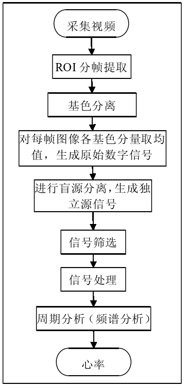
 文章介绍了利用手机摄像头进行非接触式心率测量的方法,包括录制视频、人脸校正、区域图像提取、盲源分离(ICA分析)、信号筛选和频谱分析等步骤,最终确定心率。
声明
本文在创作前已独家授权微信公众号“有晴风”进行原创发布,账号原始id为“gh_7da3ed7859e6”。文章标题为 《基于彩色视频的非接触式心率测量》
代码库
点击查看源码,欢迎star!
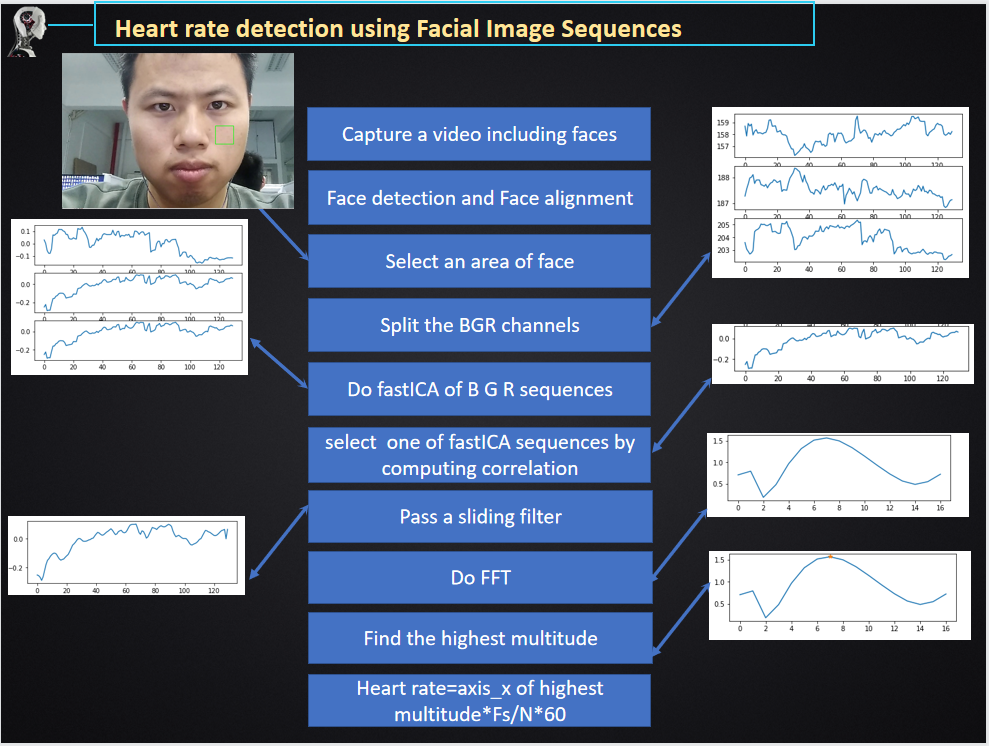
基本原理
基于彩色视频的非接触式心率测量的基本原理是:由于心脏搏动促使血液的流动,引起皮肤下的血管的容积随心脏呈脉动性变化,入射光的光程也会随之发生改变,以及血液对不同波段的光束的吸收作用不同,从而引起表层皮肤的颜色和形状变化,因此,反射光被摄像头接收到形成彩色视频图像,采集到的视频中的每帧图像在红、绿、蓝三颜色通道的亮度变化包含脉动信息,特别是绿色通道图像信号最能够反映心血管活动中心脏搏动的时间变化及其周期,即彩色视频中含有心率信息。
操作步骤
录制视频
使用手机录制即可,记得记录相机帧率,因为帧率代表着图像之间的时间间隔,需要用于测算心率。记录时尽可能保证头像不要跳出相框。
人脸校正
由于相框中的人脸还是会有一些摆动,为了消除摆动造成的图像光线变化,可以使用人脸校正算法来使面部始终保持于同一位置,便于后续区域图像截取。
人脸校正算法的大致流程是:先提取测试图像的landmark,假设为LA,然后提取待检测人脸的landmark,假设为LB,两者可通过线性变换得到,假设
L
A
=
L
B
×
W
{LA=LB \times W}
LA=LB×W
求解得到
W
{W}
W,
然后令待检测人脸的所有像素点都经过位置变换,从而得到校正后的人脸,代码如下:
import cv2
import dlib
import numpy
import os

CURRENT_PATH=os.getcwd()
PREDICTOR_PATH =CURRENT_PATH+ "/shape_predictor_68_face_landmarks.dat"
SCALE_FACTOR = 1
FEATHER_AMOUNT = 11

FACE_POINTS = list(range(17, 68))
MOUTH_POINTS = list(range(48, 61))
RIGHT_BROW_POINTS = list(range(17, 22))
LEFT_BROW_POINTS = list(range(22, 27))
RIGHT_EYE_POINTS = list(range(36, 42))
LEFT_EYE_POINTS = list(range(42, 48))
NOSE_POINTS = list(range(27, 35))
JAW_POINTS = list(range(0, 17))

# Points used to line up the images.
ALIGN_POINTS = (LEFT_BROW_POINTS + RIGHT_EYE_POINTS + LEFT_EYE_POINTS +
                               RIGHT_BROW_POINTS + NOSE_POINTS + MOUTH_POINTS)

# Points from the second image to overlay on the first. The convex hull of each
# element will be overlaid.
OVERLAY_POINTS = [
    LEFT_EYE_POINTS + RIGHT_EYE_POINTS + LEFT_BROW_POINTS + RIGHT_BROW_POINTS,
    NOSE_POINTS + MOUTH_POINTS,
]

# Amount of blur to use during colour correction, as a fraction of the
# pupillary distance.
COLOUR_CORRECT_BLUR_FRAC = 0.6

detector = dlib.get_frontal_face_detector()
predictor = dlib.shape_predictor(PREDICTOR_PATH)

class TooManyFaces(Exception):
    pass

class NoFaces(Exception):
    pass

def get_landmarks(im):
    rects = detector(im, 1)

    if len(rects) > 1:
        raise TooManyFaces
    if len(rects) == 0:
        raise NoFaces

    return numpy.matrix([[p.x, p.y] for p in predictor(im, rects[0]).parts()])

def annotate_landmarks(im, landmarks):
    im = im.copy()
    for idx, point in enumerate(landmarks):
        pos = (point[0, 0], point[0, 1])
        cv2.putText(im, str(idx), pos,
                    fontFace=cv2.FONT_HERSHEY_SCRIPT_SIMPLEX,
                    fontScale=0.4,
                    color=(0, 0, 255))
        cv2.circle(im, pos, 3, color=(0, 255, 255))
    return im

def draw_convex_hull(im, points, color):
    points = cv2.convexHull(points)
    cv2.fillConvexPoly(im, points, color=color)

def get_face_mask(im, landmarks):
    im = numpy.zeros(im.shape[:2], dtype=numpy.float64)

    for group in OVERLAY_POINTS:
        draw_convex_hull(im,
                         landmarks[group],
                         color=1)

    im = numpy.array([im, im, im]).transpose((1, 2, 0))

    im = (cv2.GaussianBlur(im, (FEATHER_AMOUNT, FEATHER_AMOUNT), 0) > 0) * 1.0
    im = cv2.GaussianBlur(im, (FEATHER_AMOUNT, FEATHER_AMOUNT), 0)

    return im

def transformation_from_points(points1, points2):
    """
    Return an affine transformation [s * R | T] such that:

        sum ||s*R*p1,i + T - p2,i||^2

    is minimized.

    """
    # Solve the procrustes problem by subtracting centroids, scaling by the
    # standard deviation, and then using the SVD to calculate the rotation. See
    # the following for more details:
    #   https://en.wikipedia.org/wiki/Orthogonal_Procrustes_problem

    points1 = points1.astype(numpy.float64)
    points2 = points2.astype(numpy.float64)

    c1 = numpy.mean(points1, axis=0)
    c2 = numpy.mean(points2, axis=0)
    points1 -= c1
    points2 -= c2

    s1 = numpy.std(points1)
    s2 = numpy.std(points2)
    points1 /= s1
    points2 /= s2

    U, S, Vt = numpy.linalg.svd(points1.T * points2)

    # The R we seek is in fact the transpose of the one given by U * Vt. This
    # is because the above formulation assumes the matrix goes on the right
    # (with row vectors) where as our solution requires the matrix to be on the
    # left (with column vectors).
    R = (U * Vt).T

    return numpy.vstack([numpy.hstack(((s2 / s1) * R,
                                       c2.T - (s2 / s1) * R * c1.T)),
                         numpy.matrix([0., 0., 1.])])

def read_im_and_landmarks(fname):
     im = cv2.imread(fname, cv2.IMREAD_COLOR)
     im = cv2.resize(im, (im.shape[1] * SCALE_FACTOR,
                         im.shape[0] * SCALE_FACTOR))

     s = get_landmarks(im)

     return im, s

def warp_im(im, M, dshape):
    output_im = numpy.zeros(dshape, dtype=im.dtype)
    cv2.warpAffine(im,
                   M[:2],
                   (dshape[1], dshape[0]),
                   dst=output_im,
                   borderMode=cv2.BORDER_TRANSPARENT,
                   flags=cv2.WARP_INVERSE_MAP)
    return output_im

def correct_colours(im1, im2, landmarks1):
    blur_amount = COLOUR_CORRECT_BLUR_FRAC * numpy.linalg.norm(
                              numpy.mean(landmarks1[LEFT_EYE_POINTS], axis=0) -
                              numpy.mean(landmarks1[RIGHT_EYE_POINTS], axis=0))
    blur_amount = int(blur_amount)
    if blur_amount % 2 == 0:
        blur_amount += 1
    im1_blur = cv2.GaussianBlur(im1, (blur_amount, blur_amount), 0)
    im2_blur = cv2.GaussianBlur(im2, (blur_amount, blur_amount), 0)

    # Avoid divide-by-zero errors.
    im2_blur += (128 * (im2_blur <= 1.0)).astype(im2_blur.dtype)

    return (im2.astype(numpy.float64) * im1_blur.astype(numpy.float64) /
                                                im2_blur.astype(numpy.float64))
#打开视频
cap=cv2.VideoCapture(CURRENT_PATH+'/my_video.mp4')
#打开校准图像
n=0
N=int(cap.get(7))
print(cap.isOpened())
im1, landmarks1 = read_im_and_landmarks(CURRENT_PATH+'/baseimg.jpg')

while (cap.isOpened()):
    ret,frame=cap.read()
    cv2.imwrite('hello.jpg',frame)
    im2, landmarks2 = read_im_and_landmarks('hello.jpg')
    cv2.imshow('capture',im2)
    cv2.waitKey(1)
    M = transformation_from_points(landmarks1[ALIGN_POINTS],
                               landmarks2[ALIGN_POINTS])

    #mask = get_face_mask(im2, landmarks2)
    #warped_mask = warp_im(mask, M, im1.shape)
    #combined_mask = numpy.max([get_face_mask(im1, landmarks1), warped_mask],
    #                      axis=0)

    warped_im2 = warp_im(im2, M, im1.shape)
   # warped_corrected_im2 = correct_colours(im1, warped_im2, landmarks1)

    #output_im = im1 * (1.0 - combined_mask) + warped_corrected_im2 * combined_mask

    cv2.imwrite(str(n)+'.jpg',warped_im2)
    n+=1
    if (n==N):
        break

cv2.destroyAllWindows()
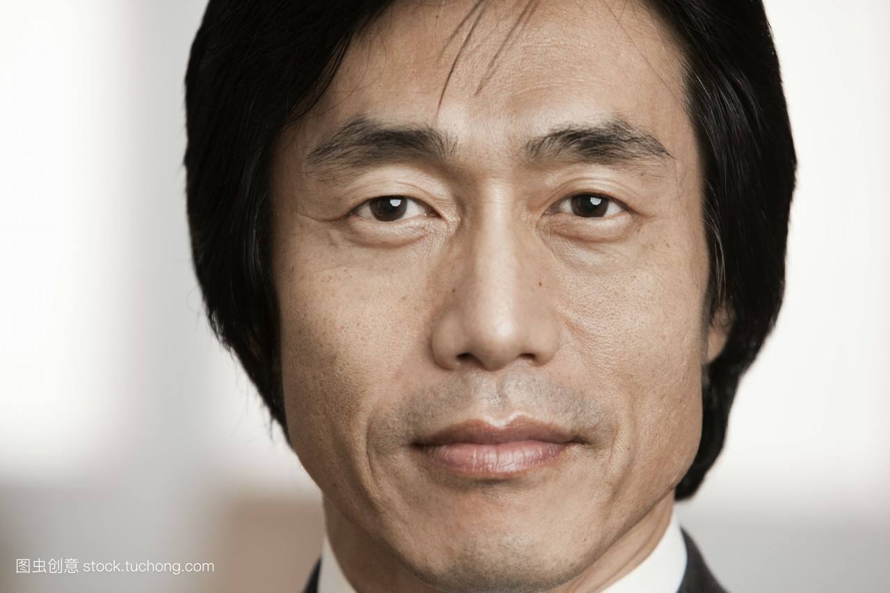
baseimg如下图:
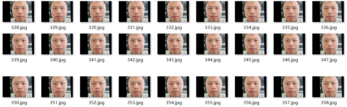
将录制的视频命名为my_video,代码运行后,得到N张校正后的人脸图像,如下图:
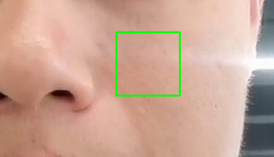
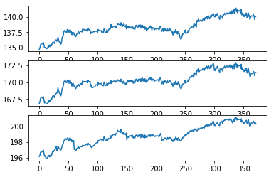
区域图像提取
在校正后的人脸上选定固定区域,提取N张小块皮肤图像,例如:
然后将每帧ROI图像进行三基色分离,生成R、G、B三通道图像,并对各通道图像所有像素取均值,将其作为该帧图像在该颜色通道的特征值,生成三个通道的数字信号
x
R
(
t
)
,
x
G
(
t
)
,
x
B
(
t
)
{x_R(t),x_G(t),x_B(t)}
xR(t),xG(t),xB(t),对这三个信号进行标准化,得到标准化的信号
x
R
(
t
)
^
,
x
G
(
t
)
^
,
x
B
(
t
)
^
{\widehat{x_R(t)},\widehat{x_G(t)},\widehat{x_B(t)}}
xR(t)
,xG(t)
,xB(t)
。
 img=image[y:y+h,x:x+w]
 xb,xg,xr=cv2.split(img)
 sum_1=0
 sum_2=0
 sum_3=0
 for i in range(xb.shape[0]):
            for j in range(xb.shape[1]):
                sum_1+=xb[i,j]
                sum_2+=xg[i,j]
                sum_3+=xr[i,j]
        sequence_b[n]=sum_1/(xb.shape[0]*xb.shape[1])
        sequence_g[n]=sum_2/(xg.shape[0]*xg.shape[1])
        sequence_r[n]=sum_3/(xr.shape[0]*xr.shape[1])
        n+=1
结果如图:
盲源分离和相关性分析
接下来,对标准化后的信号进行盲源分离(ICA分析),生成三个新的信号 y a ( t ) , y b ( t ) , y c ( t ) {y_a(t),y_b(t),y_c(t)} ya(t),yb(t),yc(t),它们之间相互独立。我的代码中使用FastICA算法进行盲源分离:
S=np.c_[sequence_b,sequence_g,sequence_r]
for i in range(N):
    S[i,:]-=np.mean(S,axis=0)
S /= S.std(axis=0)

X = np.dot(S, A.T)  # Generate observations
#Compute ICA
ica = FastICA(n_components=3)
S1= ica.fit_transform(X)  # Reconstruct signals
A_ = ica.mixing_  # Get estimated mixing matrix
assert np.allclose(X, np.dot(S1, A_.T) + ica.mean_)
结果如图:
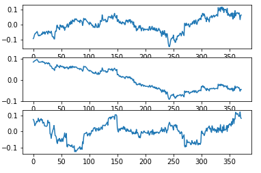
可以看到经过ICA分析之后,三个信号之间的的变化趋势明显变弱。
但由于经盲源分离(ICA分析)得到的独立源信号是无序的,无法直接选取信号,这时就需要进行信号筛选,本文采用相关性分析来进行信号筛选,通过与绿色通道信号ˆtx)(G分别做相关性分析,选取最相关的信号 y i ( t ) {y_i(t)} yi(t)其中i为a、b和c中的一个;
corr_a1=(np.corrcoef(a1,sequence_g)[0,1])
corr_a2=(np.corrcoef(a2,sequence_g)[0,1])
corr_a3=(np.corrcoef(a3,sequence_g)[0,1])
#print(corr_a1)
#print(corr_a2)
#print(corr_a3)
if (corr_a1>=corr_a2)&(corr_a1>=corr_a3): a=a1
if (corr_a2>=corr_a1)&(corr_a2>=corr_a3): a=a2
if (corr_a3>=corr_a2)&(corr_a3>=corr_a1): a=a3
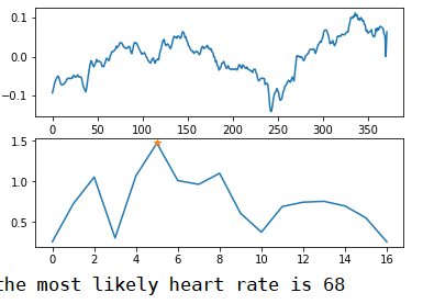
信号提取
然后需要对选取的信号进行带通滤波等信号处理;
最后对滤波后的信号作周期分析(频谱分析),即对其进行FFT变换,得到频谱图,选取最大峰值频率作为心跳频率frequency,得到心率
f
r
e
q
u
e
n
c
y
×
60
{frequency \times 60}
frequency×60。
总结
详细步骤可以简化为下图:
参考文献
[1]姚丽峰.基于PPG和彩色视频的非接触式心率测量[D].天津大学,2012.DOI:10.7666/d.D322455.
[2]Ming-Zher,Poh,Daniel,et al.Non-contact, automated cardiac pulse measurements using video imaging and blind source separation[J].Optics Express, 2010, 18(10).DOI:10.1364/oe.18.010762.


 532
532

 被折叠的 条评论
为什么被折叠?
被折叠的 条评论
为什么被折叠?
 到【灌水乐园】发言


