《机器学习实战》第三章分类

最新推荐文章于 2022-10-18 13:10:11 发布

zuckzhao95

最新推荐文章于 2022-10-18 13:10:11 发布

阅读量406

点赞数

分类专栏：《机器学习实战基于sklearn和TensorFlow》文章标签：机器学习 python

本文链接：https://blog.csdn.net/qq_35059338/article/details/107391832

版权

《机器学习实战基于sklearn和TensorFlow》专栏收录该内容

2 篇文章 0 订阅

订阅专栏

《机器学习实战》第三章分类

文章目录

《机器学习实战》第三章分类

MNIST数据集

我用的scikit-learn是0.22版本的已经取消了fetch_mldata

原书代码为：

from sklearn.datasets import fetch_mldata
mnist = fetch_mldata('MNIST original')
mnist

这样会加载不下来数据库，所以我们只能自己去网上获取数据集，让后放到工程文件里。
下载地址参考：https://blog.csdn.net/qq_30815237/article/details/87972110
下面是加载数据集的代码：

import scipy.io as scio

data_path = "mnist_dataset/mnist-original.mat"

# 获取数据集
def get_mnist_dataset(path):
    data = scio.loadmat(path)
    return data

mnist = get_mnist_dataset(data_path)
mnist

mnist = get_mnist_dataset(data_path)
X, y = mnist["data"].transpose(), mnist["label"].ravel()
X.shape, y.shape

Out：

((70000, 784), (70000,))

这里应该是数据集的格式有问题，原书中并没有使用到转置的方法。输出就是正常的（每行是一个实例，每列为单个属性），但是我下载的数据集需要转置，并且“label”标注需要用ravel()将其转为一维的数组，否则会警报，但是不会影响运行结果，建议还是降维，这样应该是更严谨的。

import numpy as np

# 划分训练集和测试集
X_train, X_test, y_train, y_test = X[:60000], X[60000:], y[:60000], y[60000:]

# 将训练集洗牌，这样能保证交叉验证时所有折叠都差不多
np.random.seed(42)
shuffle_index = np.random.permutation(60000)
X_train, y_train = X_train[shuffle_index], y_train[shuffle_index]
X_train[shuffle_index], y_train[shuffle_index]

这里训练之前，要将数据的顺序打乱，洗牌。这样能够保证交叉验证时所有的折叠都差不多。此外还有些机器学习的算法对训练实例的顺序敏感，如果连续输入相似的实例，可能导致性能不佳。

训练一个二元分类器

"""训练一个二元分类器"""
y_train_5 = (y_train == 5)  # true for all 5s, False for all other digits
y_test_5 = (y_test == 5)

from sklearn.linear_model import SGDClassifier

sgd_clf = SGDClassifier(random_state=42)
sgd_clf.fit(X_train, y_train_5)

some_digit = X[36000]
sgd_clf.predict([some_digit])

Out:

array([ True])

SGD随机梯度下降分类器，能够有效处理非常大型的数据集。SGD独立处理训练实例，一次一个，使得SGD非常适合在线学习。

性能考核

from sklearn.model_selection import StratifiedKFold
from sklearn.base import clone

skflods = StratifiedKFold(n_splits=3, shuffle=True, random_state=42)

for train_index, test_index in skflods.split(X_train, y_train_5):
    clone_clf = clone(sgd_clf)
    X_train_folds = X_train[train_index]
    y_train_folds = (y_train_5[train_index])
    X_test_fold = X_train[test_index]
    y_test_fold = (y_train_5[test_index])

    clone_clf.fit(X_train_folds, y_train_folds)
    y_pred = clone_clf.predict(X_test_fold)
    n_correct = sum(y_pred == y_test_fold)
    print(n_correct / len(y_pred))

out:

0.96815
0.92615
0.96185

sklearn.model_selection.StratifiedKFold
分层的K折交叉验证器，提供用于在训练/测试集中拆分数据集的训练/测试索引。
参数：n_splits：int类型的值，默认为5。折数
shuffle：bool类型，可选，是否在拆分之前随机排列每个类的样本。
random_state：int，随机数生成器使用的种子。
这里编译器提醒，如果设置random_state，shuffle类型必须为Ture

sklearn.base.clone
构造具有相同参数的新估算器。

利用cross_val_score()函数来评估SGDClassifier模型

from sklearn.model_selection import cross_val_score

cross_val_score(sgd_clf, X_train, y_train_5, cv=3, scoring="accuracy")

out:

array([0.9613, 0.9635, 0.9661])

精度和召回率

什么是混淆矩阵？

在这里插入图片描述

（灵敏度就是召回率）

参考链接：https://blog.csdn.net/Orange_Spotty_Cat/article/details/80520839

from sklearn.metrics import confusion_matrix

confusion_matrix(y_train_5, y_train_pred)

OUT:

array([[54122,   457],
       [ 1725,  3696]], dtype=int64)

from sklearn.metrics import precision_score, recall_score
precision_score(y_train_5, y_train_pred)

OUT：

0.8899590657356128

recall_score(y_train_5, y_train_pred)

OUT:

0.6817930271167681

这里书本上有个错误，在精度的函数中，预测结果使用了y_pred，我们知道y_pred是之前实施交叉验证时用的验证集验证的结果，y_pred的长度为2000，而y_train_5是6000长度，编译器会报valueerror

F1分数

在这里插入图片描述

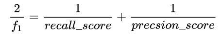
from sklearn.metrics import f1_score
f1_score(y_train_5, y_train_pred) #这里书上也写错了参数

精度/召回率均衡

y_scores = cross_val_predict(sgd_clf, X_train, y_train_5, cv=3, method="decision_function")

首先使cross_val_predic()获取训练集中所有实例的分数。

from sklearn.metrics import precision_recall_curve

precisions, recalls, thresholds = precision_recall_curve(y_train_5, y_scores)

import matplotlib.pyplot as plt

def plot_precision_recall_vs_threshold(precisions, recalls, thresholds):
    plt.plot(thresholds, precisions[:-1], "b--", label="Precision")
    plt.plot(thresholds, recalls[:-1], "g-", label="Recall")
    plt.xlabel("Threshold")
    plt.legend(loc="upper left")
    plt.ylim([0, 1])

plot_precision_recall_vs_threshold(precisions, recalls, thresholds)
plt.show()

在这里插入图片描述
ROC曲线

from sklearn.metrics import roc_curve
fpr, tpr, thresholds = roc_curve(y_train_5, y_scores)

def plot_roc_curve(fpr, tpr, label=None):
    plt.plot(fpr, tpr, linewidth=2, label=label)
    plt.plot([0, 1], [0, 1], 'k--')
    plt.axis([0, 1, 0, 1])
    plt.xlabel('False Positive Rate', fontsize=16)
    plt.ylabel('True Positive Rate', fontsize=16)

plt.figure(figsize=(8, 6))
plot_roc_curve(fpr, tpr)
plt.show()

在这里插入图片描述

随机森林分类器

from sklearn.ensemble import RandomForestClassifier
forest_clf = RandomForestClassifier(random_state=42)
y_probas_forest = cross_val_predict(forest_clf, X_train, y_train_5, cv=3, method="predict_proba")

y_scores_forest = y_probas_forest[:, 1]
fpr_forest, tpr_forest, thresholds_forest = roc_curve(y_train_5, y_scores_forest)

plt.plot(fpr, tpr, "b:", label="SGD")
plot_roc_curve(fpr_forest, tpr_forest, "Random Forest")
plt.legend(loc="lower right")  # 这里原书是bottom right，但我的0.22版本中只能写lower right
plt.show()

多类别分类器

解决多分类问题，一般有两种思路：
一种叫做一对多策略（OvA），就是每个类别训练一个估算器，然后对一个实例预测时，分别应用所有类别的估算器，哪个分类器给出的分最高，就分为哪一类；
另一种叫做一对一策略（OvO），这个OvO很像表情如果存在N个类别，就训练N*(N-1)/2个分类器，两两进行分类，需要对一个实例进行分类时，需要运行所有的分类器，就像两个两个打循环赛一样，最后获胜次数最多的类别，就将实例划分为此类。

Sklearn检测到多类别分类任务时，可以自动运行OvA（SVM除外）

sgd_clf.fit(X_train, y_train)
sgd_clf.predict([some_digit])

OUT：array([5.])

some_digit_scores = sgd_clf.decision_function([some_digit])
some_digit_scores

OUT:

array([[ -8204.47519778, -19206.28224706,  -5702.10113982,
         -4666.3653033 , -15827.7809826 ,   1782.52380291,
        -39807.3747045 , -18945.8333413 , -14650.34384565,
        -16166.06981109]])

sgd_clf.classes_

OUT：

array([0., 1., 2., 3., 4., 5., 6., 7., 8., 9.])

如何使用OvO分类

from sklearn.multiclass import OneVsOneClassifier
ovo_clf = OneVsOneClassifier(SGDClassifier(random_state=42))
ovo_clf.fit(X_train, y_train)
ovo_clf.predict([some_digit])

OUT：array([5.])

len(ovo_clf.estimators_)

OUT：45

cross_val_score(sgd_clf, X_train, y_train, cv=3, scoring="accuracy")

OUT：array([0.88875, 0.8722 , 0.87905])

使用标准化将输入数据简单缩放，可以提高准确率

from sklearn.preprocessing import StandardScaler
scaler = StandardScaler()
X_train_scaled = scaler.fit_transform(X_train.astype(np.float64))
cross_val_score(sgd_clf, X_train_scaled, y_train, cv=3, scoring="accuracy")

OUT：array([0.9044, 0.9005, 0.9003])

错误分析

y_train_pred = cross_val_predict(sgd_clf, X_train_scaled, y_train, cv=3)
conf_mx = confusion_matrix(y_train, y_train_pred)
conf_mx

OUT：

array([[5605,    0,   13,    9,   10,   44,   37,    6,  198,    1],
       [   1, 6425,   41,   20,    3,   41,    4,    8,  187,   12],
       [  26,   26, 5256,   86,   71,   26,   69,   41,  347,   10],
       [  31,   21,  113, 5256,    2,  206,   29,   44,  363,   66],
       [  11,   16,   36,   10, 5254,    9,   42,   19,  273,  172],
       [  31,   21,   22,  160,   53, 4485,   79,   20,  484,   66],
       [  29,   18,   45,    3,   36,   91, 5567,    5,  124,    0],
       [  23,   12,   54,   29,   50,   12,    5, 5703,  151,  226],
       [  20,   69,   38,  106,    1,  122,   30,   10, 5407,   48],
       [  24,   22,   28,   57,  131,   35,    1,  183,  322, 5146]],
      dtype=int64)

plt.matshow(conf_mx, cmap=plt.cm.gray)
plt.show()

在这里插入图片描述

row_sums = conf_mx.sum(axis=1, keepdims=True)
norm_conf_mx = conf_mx / row_sums

np.fill_diagonal(norm_conf_mx, 0)
plt.matshow(norm_conf_mx, cmap=plt.cm.gray)
plt.show()

$[外链图片转存失败,源站可能有防盗链机制,建议将图片保存下来直接上传(img-RBZULSrR-1594900184128)(F:\WorkSpace\学习日记\hands on ML\classification.assets\image-20200716174819594.png)]$

zuckzhao95

关注

0
点赞
踩
0

收藏

觉得还不错? 一键收藏
0
评论
《机器学习实战》第三章分类

《机器学习实战》第三章分类文章目录《机器学习实战》第三章分类MNIST数据集训练一个二元分类器性能考核精度和召回率在这里插入图片描述多类别分类器错误分析MNIST数据集我用的scikit-learn是0.22版本的已经取消了fetch_mldata原书代码为：from sklearn.datasets import fetch_mldatamnist = fetch_mldata('MNIST original')mnist这样会加载不下来数据库，所以我们只能自己去网上获取数据集，让后
复制链接

扫一扫