


数据

将数据保存到txt文件中,如下图所示,最后一列代表类别
批更新 感知机 算法实现
import numpy as np
import matplotlib.pyplot as plt
def batch_perception(data,yt,w1,w2):
a = np.array([[0, 0, 0]])
w1 = str(w1)
w2 = str(w2)
#散点图绘制
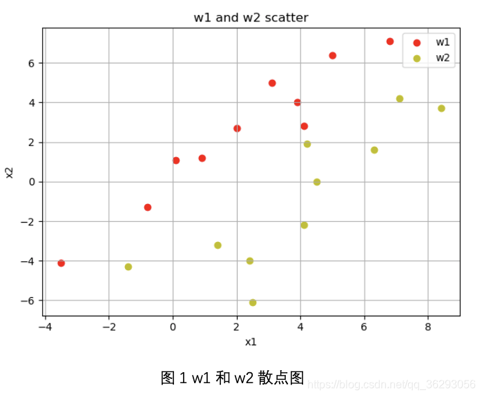
plt.scatter(data[0:10, 0], data[0:10, 1], c='r', label='w'+w1)
plt.scatter(data[10:20, 0], data[10:20, 1], c='y', label='w'+w2)
plt.xlabel('x1')
plt.ylabel('x2')
plt.title('w'+w1+' and '+'w'+w2+' scatter')
plt.legend()
plt.grid(True)
plt.show()
y = np.ones(data.shape)
y[:, 0:2] = data[:, 0:2]
#规范化
y[10:20, :] = -y[10:20, :]
f = 1
c = 0
while f != 0:
g = np.dot(a, y.T)
fn = y[np.argwhere(g[0] <= 0)]
for i in range (fn.shape[0]):
a = a+yt*fn[i, :]
f = fn.shape[0]
# 记录收敛次数
c += 1
#绘制决策面
plt.scatter(data[0:10, 0], data[0:10, 1], c='r', label='w'+w1)
plt.scatter(data[10:20, 0], data[10:20, 1], c='y', label='w'+w2)
plt.plot(data[:, 0], -(a[0][0]*data[:, 0]+a[0][2]*1)/a[0][1], label='decision boundary')
plt.xlabel('x1')
plt.ylabel('x2')
plt.title('w'+w1+' and '+'w'+w2+' decision boundary')
plt.legend()
plt.grid(True)
plt.show()
return a, c
if __name__ == '__main__':
data = np.loadtxt('data.txt')
[a1, c1] = batch_perception(data[0:20, :],0.01,1,2)
[a2, c2] = batch_perception(data[10:30, :],0.01,2,3)
print(c1)
print(c2)
运行结果
收敛步数:24

收敛次数 17

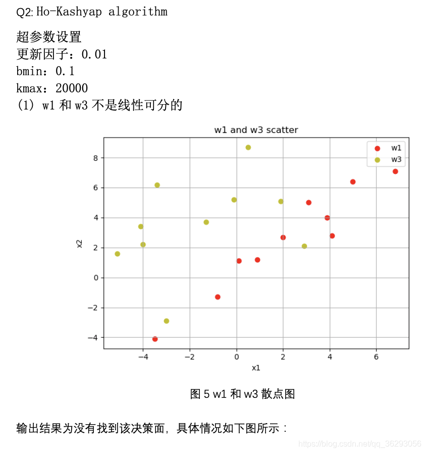
Ho-Kashyap algorithm
import numpy as np
import matplotlib.pyplot as plt
def isBreak(x, y):
for i in range(x.shape[1]):
if x[0][i] > y:
return False
return True
def Ho_Kashyap(data, yt,w1,w2):
w1 = str(w1)
w2 = str(w2)
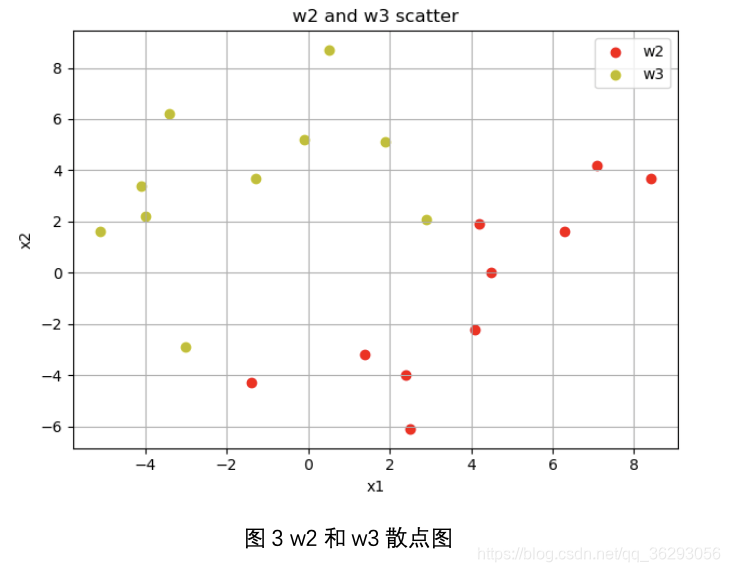
plt.scatter(data[0:10, 0], data[0:10, 1], c='r', label='w'+w1)
plt.scatter(data[10:20, 0], data[10:20, 1], c='y', label='w'+w2)
plt.xlabel('x1')
plt.ylabel('x2')
plt.title('w' + w1 + ' and ' + 'w' + w2 + ' scatter')
plt.legend()
plt.grid(True)
plt.show()
y = np.ones(data.shape)
y[:, 0:2] = data[:, 0:2]
y[10:20, :] = -y[10:20, :]
a = np.zeros([1, 3])
n = data.shape[0]
b = np.ones([1, n])*0.5
bmin = 0.1
kmax = 20000
k = 0
while k < kmax:
e = np.dot(a, y.T)-b
e1 = 1/2*(e+np.abs(e))
b = b+2*yt*e1
a = np.dot(b, np.linalg.pinv(y.T))
if isBreak(np.abs(e), bmin):
return [a, b, e]
k = k+1
print("未找到")
return None
def pic(data, a, b, w1,w2):
w1 = str(w1)
w2 = str(w2)
plt.scatter(data[0:10, 0], data[0:10, 1], c='r', label='w' + w1)
plt.scatter(data[10:20, 0], data[10:20, 1], c='y', label='w' + w2)
plt.legend()
plt.plot(data[:, 0], -(a[0][0] * data[:, 0] + a[0][2] * 1) / a[0][1], label='decision boundary')
plt.xlabel('x1')
plt.ylabel('x2')
plt.title('ho kashyap '+'w' + w1 + ' and ' + 'w' + w2 + ' decision boundary')
plt.legend()
plt.grid(True)
plt.show()
def as_num(x):
y='{:.12f}'.format(x)
return(y)
if __name__ == '__main__':
data = np.loadtxt('data.txt')
data1 = np.vstack((data[0:10, :], data[20:30, :]))
data2 = np.vstack((data[10:20, :], data[30:40, :]))
x1 = Ho_Kashyap(data1, 0.01, 1, 3)
x2 = Ho_Kashyap(data2, 0.01, 2, 4)
if x1 != None:
pic(data1, x1[0], x1[1], 1, 3)
print(x1[2])
if x2 != None:
pic(data2, x2[0], x2[1], 2, 4)
print(x2[2])
运行结果

MSE
import numpy as np
import matplotlib.pyplot as plt

class MSE():

    def process(self,data,c):
        n = data.shape[0]
        c1 = c.shape[0]
        y_label = np.zeros([n, c1])
        index = data[:, 2]-1
        for i in range(data.shape[0]):
            y_label[i, int(index[i])] = 1
        x = np.ones((n, 3))
        x[:, 0:2] = data[:, 0:2]
        return x, y_label

    def MSE_train(self, data_train, c):
        x, y_label = self.process(data_train, c)
        w = np.ones_like(x.T)
        w = np.matmul(np.linalg.pinv(x), y_label)
        self.w = w

    def MSE_test(self, data_test, c):
        x, y_label = self.process(data_test,c)
        y_test = np.matmul(self.w.T, x.T)
        correct = np.sum(np.argmax(y_test.T, axis=1)==np.argmax(y_label,axis=1))/len(y_label)
        return correct


if __name__ == '__main__':
    data = np.loadtxt("data.txt")
    for i in range(4):
        if i == 0:
            data_train = data[i*10:i*10+8, :]
            data_test = data[i*10+8:i*10+10, :]
        if i != 0:
            data_train = np.append(data_train, data[i*10:i*10+8, :], axis=0)
            data_test = np.append(data_test, data[i*10+8:i*10+10, :], axis=0)
    c = np.array([1,2,3,4])
    M = MSE()
    M.MSE_train(data_train,c)
    correct = M.MSE_test(data_test,c)
    print('测试样本正确率:',correct)
运行结果


 1717
1717


 被折叠的 条评论
为什么被折叠?
被折叠的 条评论
为什么被折叠?
 到【灌水乐园】发言


