


python实现SVM分类且进行调参
问题描述
从 MNIST 数据集中任意选择两类,对其进行 SVM 分类,可调用现有的 SVM 工具如 LIBSVM,展示超参数 C 以及核函数参数的选择过程。
求解过程
第一步:数据集下载,代码如下:
mnist = tf.keras.datasets.mnist
(x_train, y_train), (x_test, y_test) = mnist.load_data()
第二步:选定核函数为 RBF
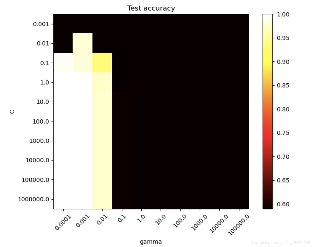
第三步:手动进行调参,调参过程如下,显示的准确率是测试集的,可以看出当 gamma 的值为 0.0001、0.001;C 的值为 0.1 以上时泛化性能较好。
手动调参的代码
from sklearn import svm
import numpy as np
import tensorflow as tf
from sklearn.preprocessing import StandardScaler
import matplotlib.pyplot as plt
import time
mnist = tf.keras.datasets.mnist

(x_train, y_train), (x_test, y_test) = mnist.load_data()
x_train, x_test = x_train / 255.0, x_test / 255.0
x_train = x_train.reshape([x_train.shape[0], -1])
x_test = x_test.reshape([x_test.shape[0], -1])
train_x = []
train_y = []
for i in range(x_train.shape[0]):
    if y_train[i] == 0 or y_train[i] == 1:
        train_x.append(x_train[i])
        train_y.append(y_train[i])
train_x = np.array(train_x)
train_y = np.array(train_y)
test_x = []
test_y = []
for i in range(x_test.shape[0]):
    if y_test[i] == 0 or y_test[i] == 1:
        test_x.append(x_test[i])
        test_y.append(y_test[i])
test_x = np.array(test_x)
test_y = np.array(test_y)
train_x = train_x[0:1000]
train_y = train_y[0:1000]
test_x = test_x[0:300]
test_y = test_y[0:300]
scaler = StandardScaler()
train_x = scaler.fit_transform(train_x)
test_x = scaler.fit_transform(test_x)


score = np.zeros([10,10])
C_range = np.logspace(-3, 6, 10)
gamma_range = np.logspace(-4, 5, 10)
for i,c in enumerate(C_range):
    for j,g in enumerate(gamma_range):
        start = time.time()
        svc = svm.SVC(C=c, kernel='rbf', gamma=g, decision_function_shape='ovo')
        svc.fit(train_x, train_y)
        score[i,j] = svc.score(test_x, test_y)
        end = time.time()
        print('c:',c,'g:',g,'time:',(end-start))


plt.figure(figsize=(8, 6))
plt.subplots_adjust(left=.2, right=0.95, bottom=0.15, top=0.95)
plt.imshow(score, interpolation='nearest', cmap=plt.cm.hot)
plt.xlabel('gamma')
plt.ylabel('C')
plt.colorbar()
plt.xticks(np.arange(len(gamma_range)), gamma_range, rotation=45)
plt.yticks(np.arange(len(C_range)), C_range)
plt.title('Test accuracy')
plt.show()
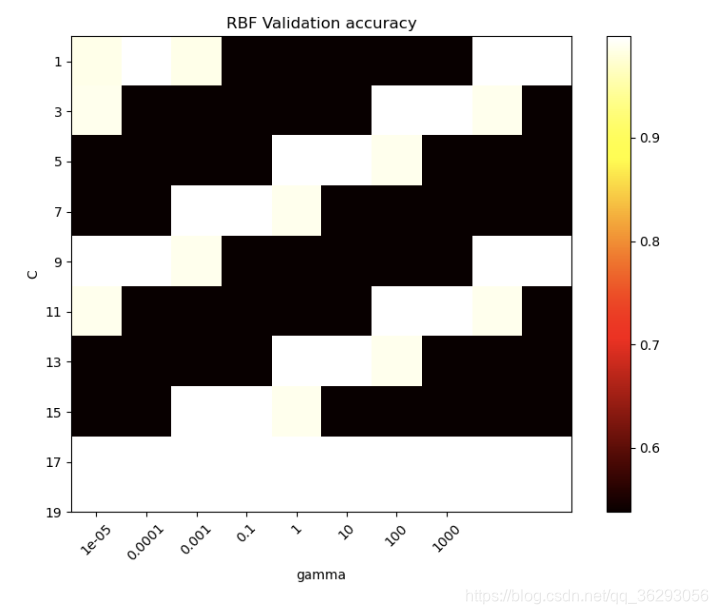
第四步:网格调参,参数如下
输出为:The best parameters are {‘C’: 3, ‘gamma’: 0.0001, ‘kernel’: ‘rbf’} with a score of 1.00
代码
from sklearn import svm
import numpy as np
import tensorflow as tf
from sklearn.preprocessing import StandardScaler
import matplotlib.pyplot as plt
from sklearn.model_selection import GridSearchCV
mnist = tf.keras.datasets.mnist
(x_train, y_train), (x_test, y_test) = mnist.load_data()
x_train, x_test = x_train / 255.0, x_test / 255.0
x_train = x_train.reshape([x_train.shape[0], -1])
x_test = x_test.reshape([x_test.shape[0], -1])
train_x = []
train_y = []
for i in range(x_train.shape[0]):
    if y_train[i] == 0 or y_train[i] == 1:
        train_x.append(x_train[i])
        train_y.append(y_train[i])
train_x = np.array(train_x)
train_y = np.array(train_y)
test_x = []
test_y = []
for i in range(x_test.shape[0]):
    if y_test[i] == 0 or y_test[i] == 1:
        test_x.append(x_test[i])
        test_y.append(y_test[i])
test_x = np.array(test_x)
test_y = np.array(test_y)
train_x = train_x[0:1000]
train_y = train_y[0:1000]
test_x = test_x[0:300]
test_y = test_y[0:300]
scaler = StandardScaler()
train_x = scaler.fit_transform(train_x)
test_x = scaler.fit_transform(test_x)

parameters = [
	{
		'C': [1, 3, 5, 7, 9, 11, 13, 15, 17, 19],
	    'gamma': [0.00001, 0.0001, 0.001, 0.1, 1, 10, 100, 1000],
	    'kernel': ['rbf']
	},
	{
		'C': [1, 3, 5, 7, 9, 11, 13, 15, 17, 19],
	    'kernel': ['linear']
	}
]

svc = svm.SVC()
clf = GridSearchCV(svc, parameters, cv=3, n_jobs=8)
clf.fit(train_x,train_y)

print("The best parameters are %s with a score of %0.2f"
      % (clf.best_params_, clf.best_score_))

scores = clf.cv_results_['mean_test_score'][0:80].reshape(8,10)

plt.figure(figsize=(8, 6))
plt.subplots_adjust(left=.2, right=0.95, bottom=0.15, top=0.95)
plt.imshow(scores, interpolation='nearest', cmap=plt.cm.hot)
plt.xlabel('gamma')
plt.ylabel('C')
plt.colorbar()
plt.xticks(np.arange(8), [0.00001, 0.0001, 0.001, 0.1, 1, 10, 100, 1000], rotation=45)
plt.yticks(np.arange(10), [1, 3, 5, 7, 9, 11, 13, 15, 17, 19])
plt.title('RBF Validation accuracy')
plt.show()
说明
tensorflow==2.4


 被折叠的 条评论
为什么被折叠?
被折叠的 条评论
为什么被折叠?
 到【灌水乐园】发言


