5.逻辑回归

`
import numpy as np
import matplotlib.pyplot as plt
#评估模型
from sklearn.metrics import classification_report
from sklearn import preprocessing
#数据是否需要标准化
scale = False
#scale = True
import numpy as np
import matplotlib.pyplot as plt
#评估模型
from sklearn.metrics import classification_report
from sklearn import preprocessing
#数据是否需要标准化
scale = False
#scale = True
In [13]:

#载入数据
data = np.genfromtxt(r"LR-testSet.csv",delimiter=",")
#print(data)
x_data = data[:,:-1]
#print(x_data)
y_data = data[:,-1]
#print(y_data)
​
#画图函数
def plot():
x0 = []
x1 = []
y0 = []
y1 = []
#切分不同类别的数据
for i in range(len(x_data)):
if y_data[i] == 0:
x0.append(x_data[i,0])
y0.append(x_data[i,1])
else :
x1.append(x_data[i,0])
y1.append(x_data[i,1])
#画图
scatter0 = plt.scatter(x0,y0, c=‘b’, marker=‘o’)
scatter1 = plt.scatter(x1,y1, c=‘r’, marker=‘x’)

#画图例
plt.legend(handles=[scatter0,scatter1],labels=['labels0','labels1'], loc='best')

plot()
plt.show()

In [17]:

#数据处理
x_data = data[:,:-1]
y_data = data[:,-1,np.newaxis]
​
print(np.mat(x_data).shape)
print(np.mat(y_data).shape)
​
#给样本添加偏置项
X_data = np.concatenate((np.ones((100,1)),x_data),axis=1)
print(X_data.shape)
(100, 2)
(100, 1)
(100, 3)
In [25]:

记录
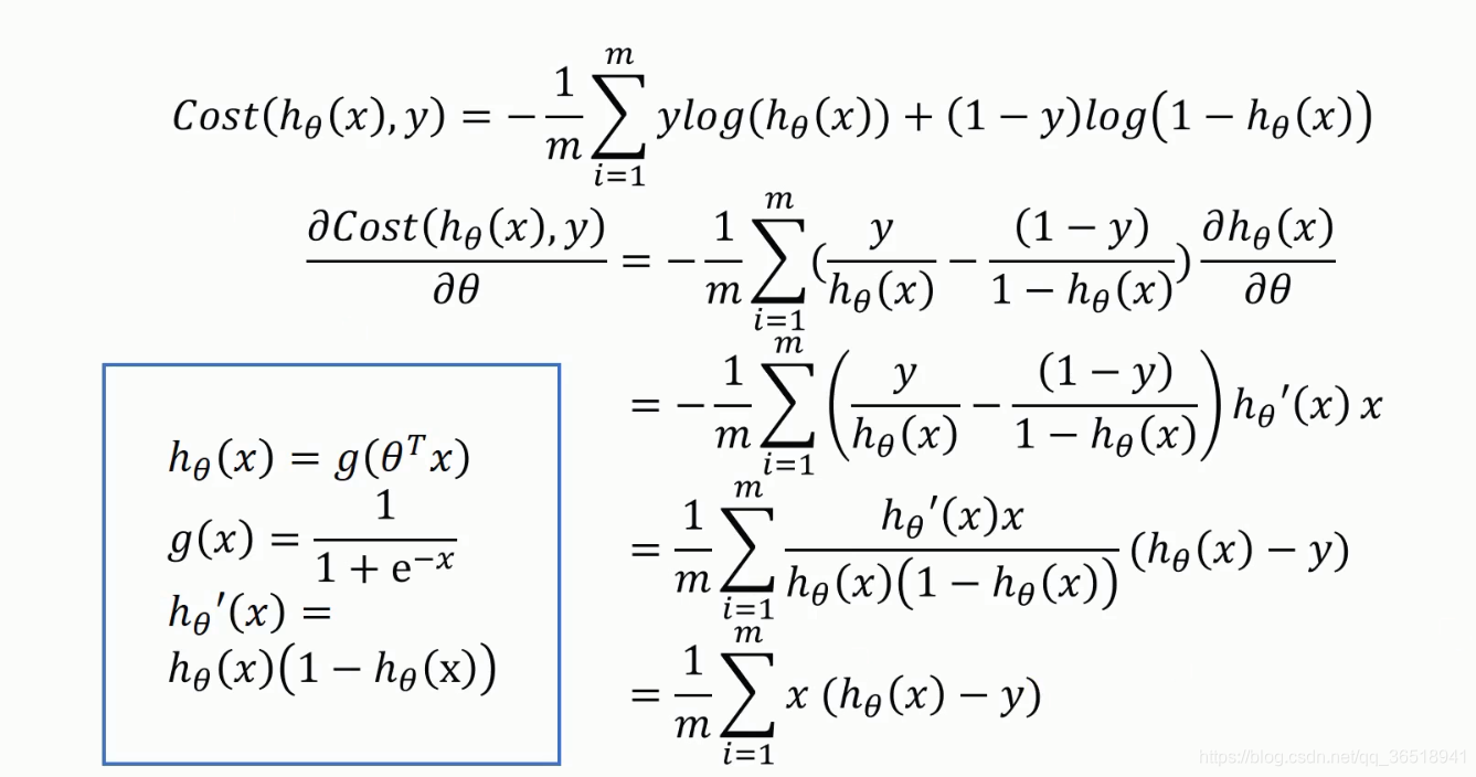
#逻辑回归函数
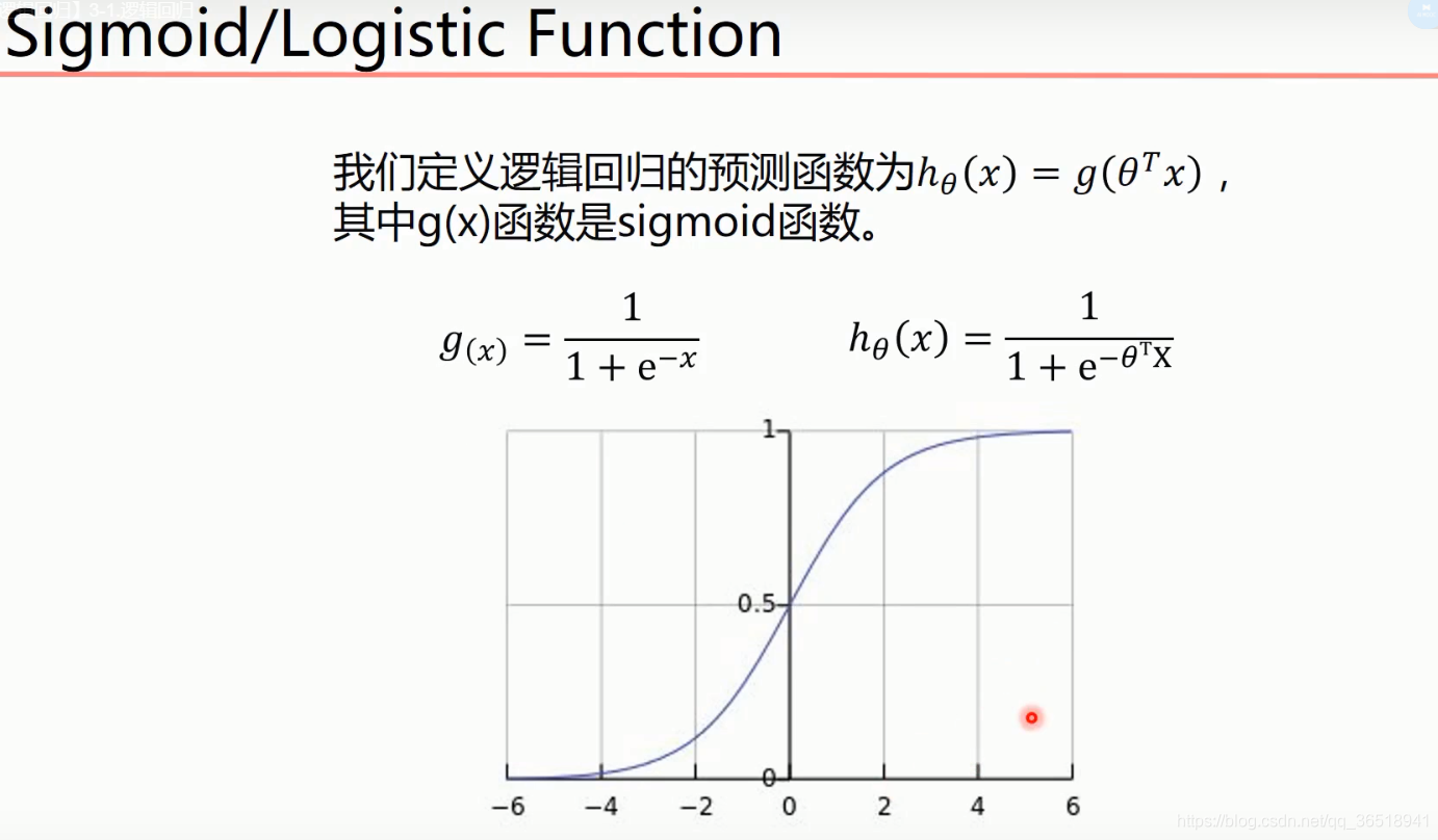
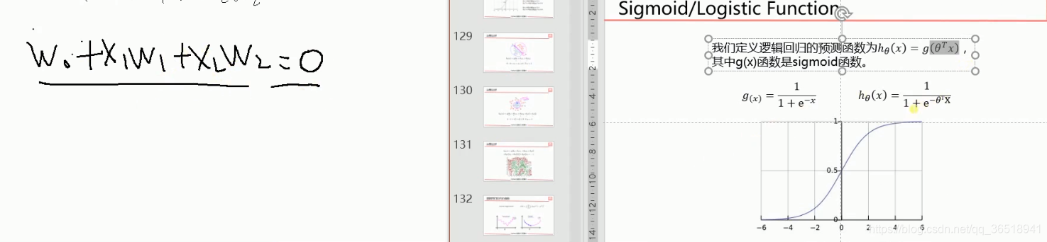
def sigmoid(x):
return 1.0/(1+np.exp(-x))
​
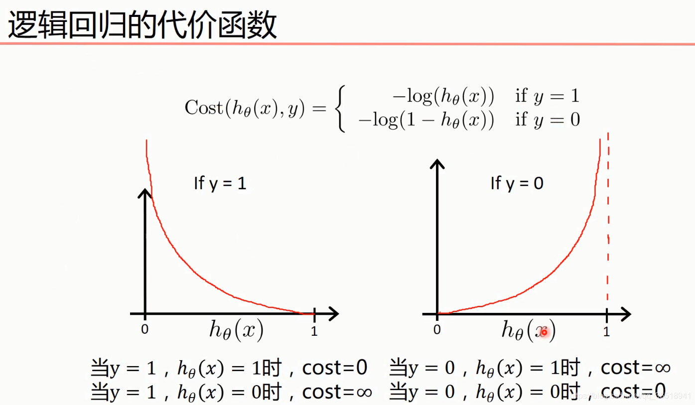
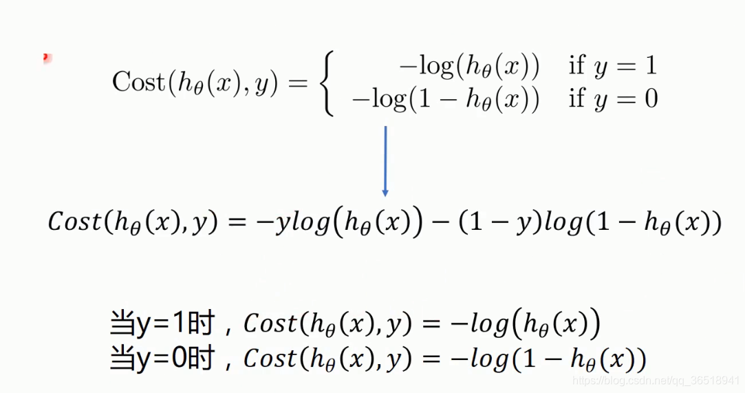
#逻辑回归的代价函数
def cost(xMat, yMat, ws):
#multiply:按位相乘
left = np.multiply(yMat, np.log(sigmoid(xMat * ws)))
right = np.multiply(1 - yMat,np.log(1-sigmoid(xMat*ws)))
return np.sum(left+right) / -(len(xMat))
​
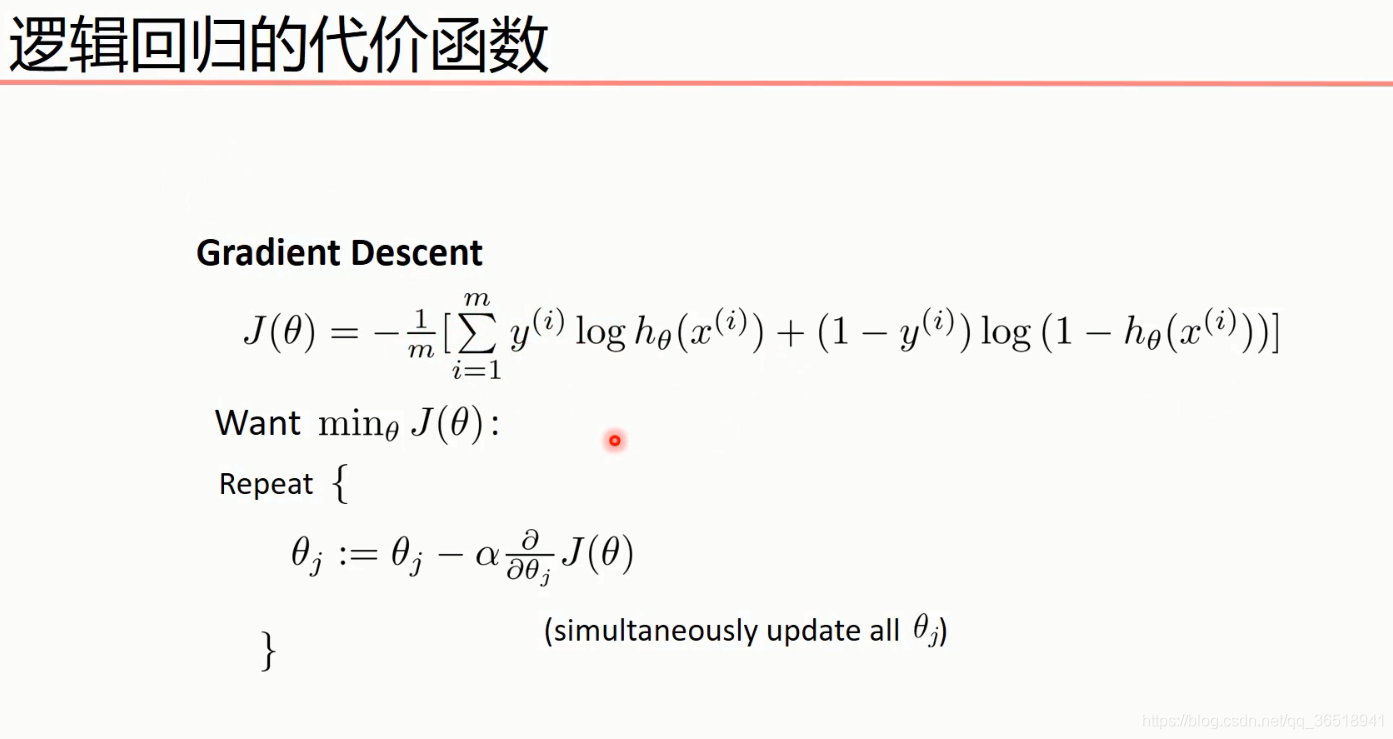
def gradAscent(xArr, yArr):
if scale == True:
xArr = preprocessing.scale(xArr)
xMat = np.mat(xArr)
yMat = np.mat(yArr)

#学习率
lr = 0.001
#迭代次数
epochs = 10000
costlist = []
#计算数据行列数
#行代表数据个数， 列代表权值个数
m,n = np.shape(xMat)#100,3
#初始化权值,3个特征代表3个权值
ws = np.mat(np.ones((n,1)))

for i in range(epochs+1):
    #xMat和weights矩阵相乘
    h = sigmoid(xMat * ws)#h是矩阵的形式
    
    #计算误差
    ws_grad = xMat.T *(h-yMat)/m
    ws= ws- lr* ws_grad
    
    if i%50 == 0:#一共记录201次
        costlist.append(cost(xMat,yMat,ws))
return ws,costlist

In [27]:

#训练模型，得到权值和cost值的变化
ws, costlist = gradAscent(X_data, y_data)
print(ws)
[[ 2.05836354]
[ 0.3510579 ]
[-0.36341304]]
In [29]:

#画图
if scale == False:
#画出决策边界
plot()
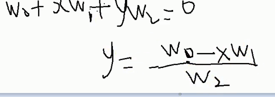
x_test = [[-4],[3]]
y_test =(-ws[0] - x_test*ws[1])/ws[2]
plt.plot(x_test, y_test,‘k’)
plt.show()

In [32]:

#画图 loss值的变化
x = np.linspace(0,10000,201)
plt.plot(x,costlist,c=‘r’)
plt.title(‘train’)
plt.xlabel(‘Epochs’)
plt.ylabel(‘Cost’)
plt.show()

In [35]:

)
#预测
def predict(x_data, ws):#返回List数组，0或者1
if scale ==True:
x_data = preprocessing.scale(x_data)#便准化
xMat = np.mat(x_data)
ws = np.mat(ws)
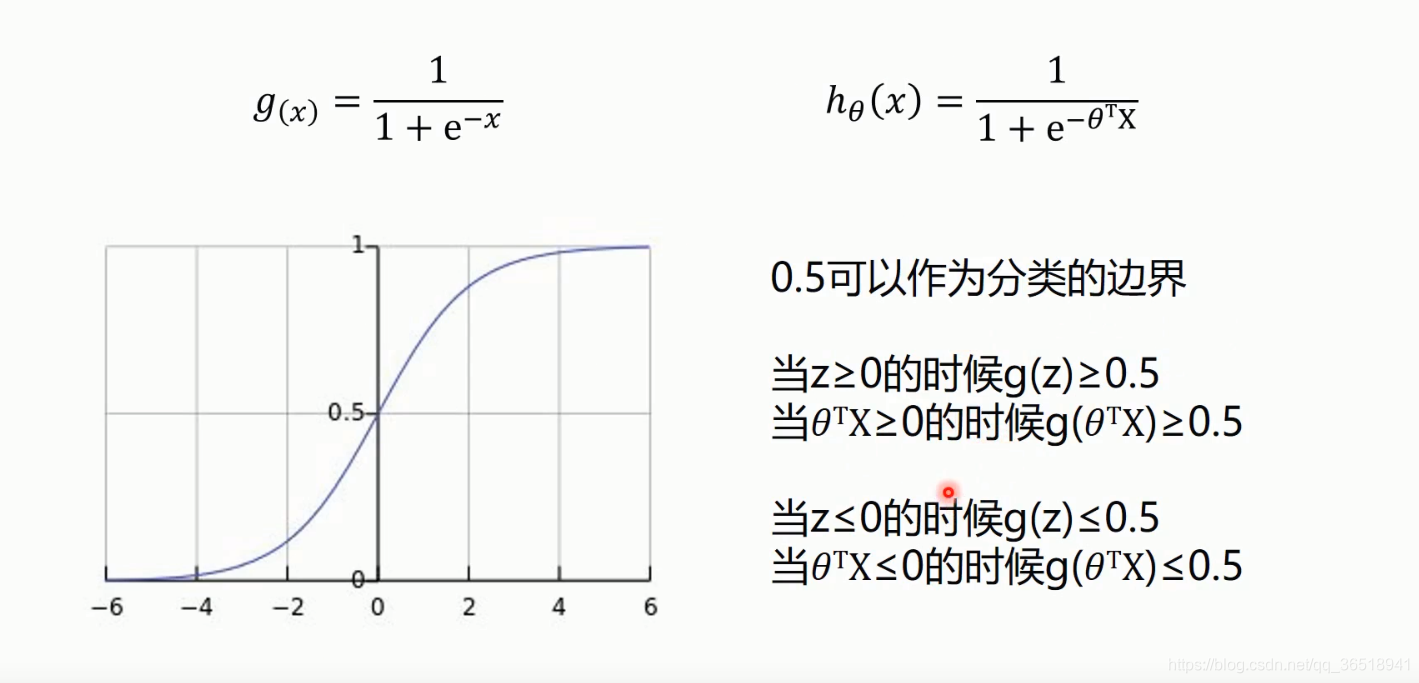
return [1 if x>=0.5 else 0 for x in sigmoid(xMat * ws)]
predictions = predict(X_data,ws)
print(classification_report(y_data,predictions))
precision recall f1-score support

    0.0       0.82      1.00      0.90        47
    1.0       1.00      0.81      0.90        53

avg / total 0.92 0.90 0.90 100

In [ ]:

​
`