


摘要
基于凯斯西厨大学的轴承数据,首先利用数据增强方法,对原始数据进行重叠采样,增加样本数量。然后,利用连续小波变换,将一维的训练样本转换为二维RGB图像。其次,将处理好的样本进行样本分割为训练集、测试集,输入到卷积神经网络训练。最后,利用T-SNE降维算法对模型指定网络层进行动态可视化显示。
数据集
引入了由美国凯斯西储大学(CWRU)数据中心获得的轴承故障基准数据集。采用实验试验台(如图1所示)对轴承缺陷检测信号进行检测。该平台由一个 1.5W 的电动机(左)、扭矩传感器译码器(中)和一个功率测试计(右)组成。通过使用电火花加工对轴承造成损伤,损伤的位置分别为外圈、内圈和滚动体。其中轴承有两种型号,一种是放置在驱动端的轴承,型号为 SKF6205,采样频率为12Khz 和 48Khz。另一种是放置在风扇端的轴承,型号为 SKF6203,采样频率为12Khz。振动信号的采集由加速度计来完成。本文研究所使用的数据均来自采样频率为12Khz的驱动端轴承。同时,实验采用的轴承故障直径为0.007英寸、0.014英寸和0.021英寸。
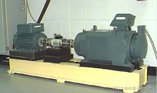
图1 凯斯西储大学轴承数据
西储大学下载地址:http://csegroups.case.edu/bearingdatacenter/pages/download-data-file
上面是官方给的数据,自己下载下来,根据自己的需要进行整理归类。下面是我自己整理的数据文件夹。07、14、21是三种轴承尺寸;0、1、2、3是4种不同负载;1797、1772、1750、1797对4种不同负载的速度。如图2所示。
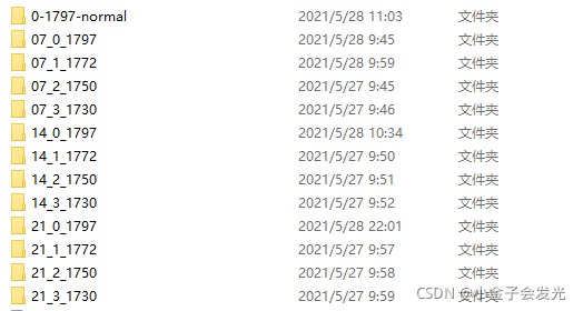
图2 数据类型数据整理
数据预处理
数据预处理部分,利用matlab进行数据增强、连续小波变化。
1.数据增强
深度学习虽具有很好的学习能力,但通常也有一个弊端:需要在数据量比较大的前提下才能取到一个较好的效果。考虑到每一种轴承故障类型中振动信号的个数只有12万个多,按照1024个振动信号点作为一个样本,最多只有 120 个样本。因此为了增强模型的泛化性和鲁棒性,使用数据增强方法对数据集进行扩充。简单粗暴理解,好比切西瓜,本来一块很大的西瓜,被你按照一定距离、方向切了很多刀,成了好几块均匀的西瓜。
原理参考:基于深度学习的轴承故障识别-数据预处理_轴承故障数据预处理_zhangjiali12011的博客-CSDN博客
2.连续小波变换
和短时傅里叶变换相比,小波变换有着窗口自适应的特点,即高频信号分辨率高(但是频率分辨率差),低频信号频率分辨率高(但是时间分辨率差),而在工程中常常比较关心低频的频率,关心高频出现的时间,所以近些年用途比较广泛。简单粗暴理解,将本来一维的数据变成二维的图像。
原理参考:https://blog.csdn.net/weixin_42943114/article/details/896032
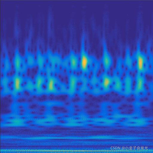
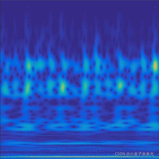
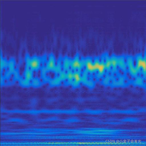
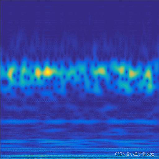
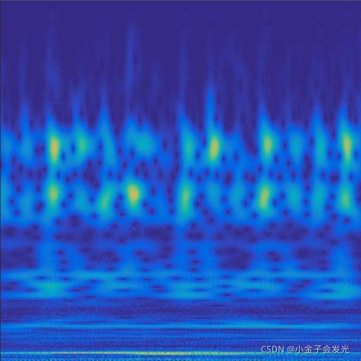
3.效果展示
由于自己电脑配置有限,计算速度各方面还是有点不足,仅仅做了6类故障诊断。如图3所示。
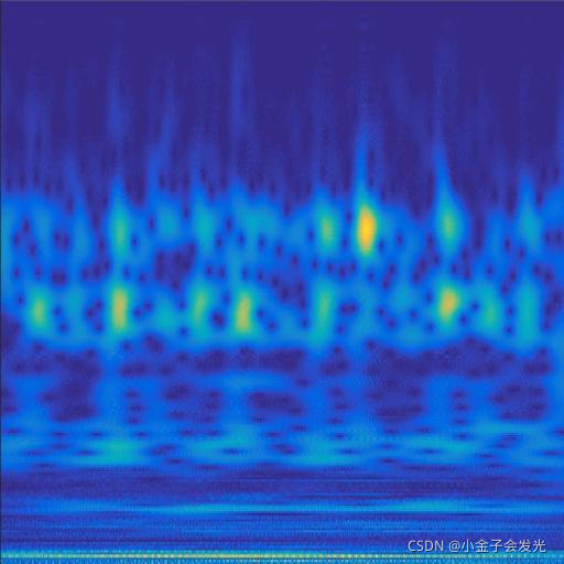
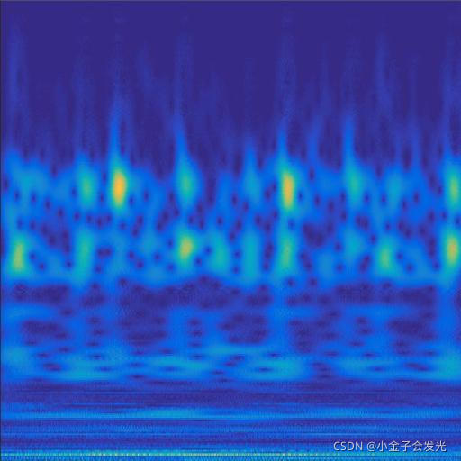
105inner数据
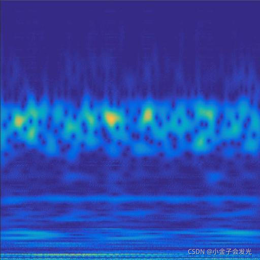
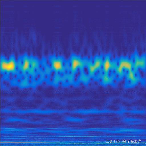
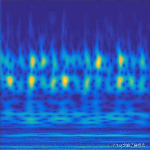
118ball数据
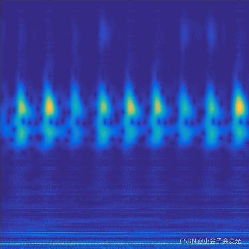
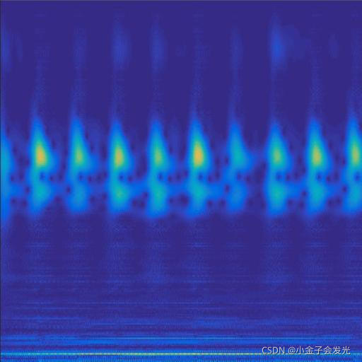
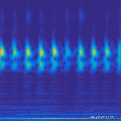
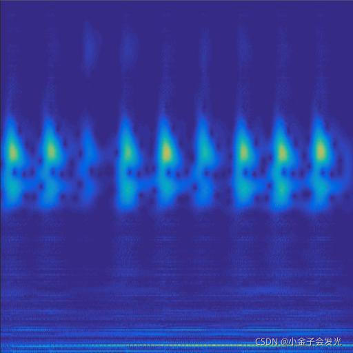
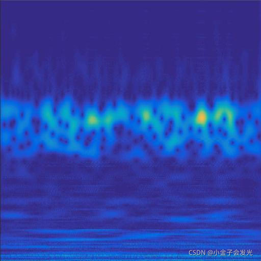
130outer数据
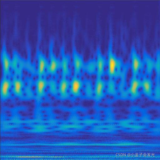
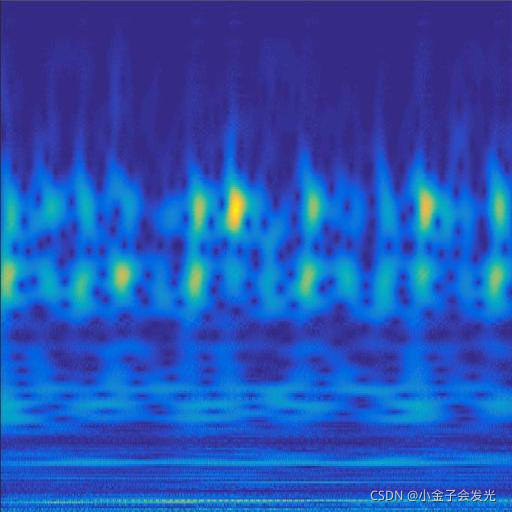
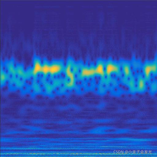
119ball数据
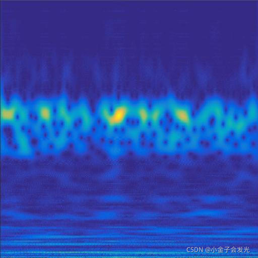
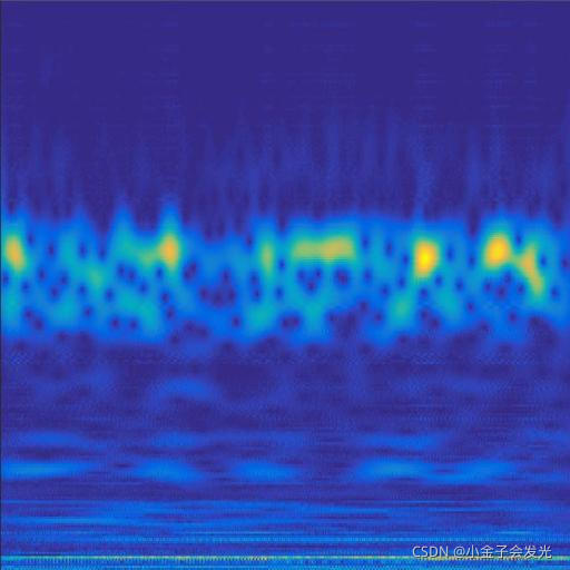
119inner数据
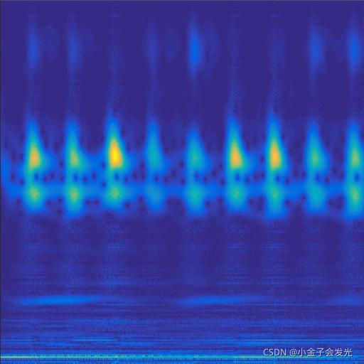
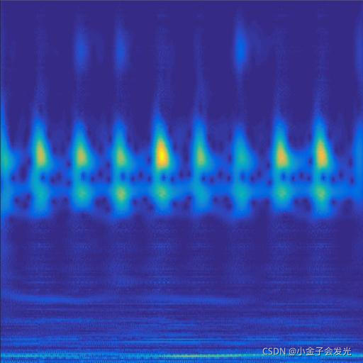
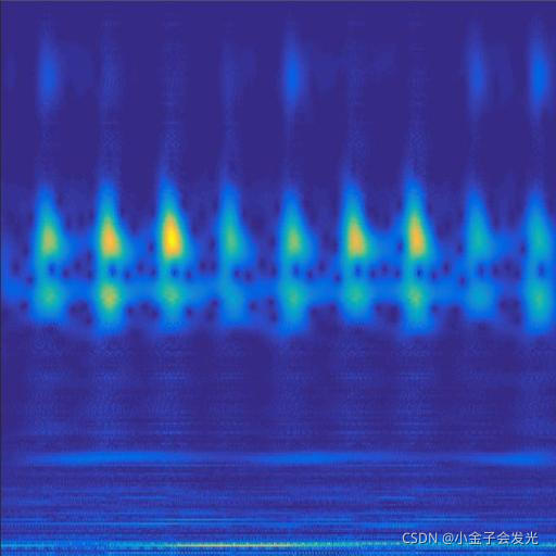
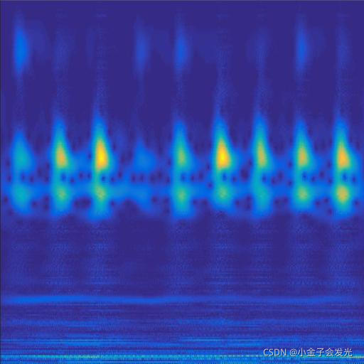
131outer数据
图3 六种小波变换效果
模型训练
VGG16卷积神经网络结构如图4所示,通过反复叠加的卷积层(convolution layer)和池化层(pooling layer),共有13层卷积层和3层全连接层(fully connected layer),而池化层不计权重故不算在总层数之内。卷积层和池化层其实就是对输入图像的一种提取过程,多层卷积池化层相互堆叠,使得网络具有更大感受野的同时又能降低网络参数,并且通过ReLU激活函数使得原本的单一线性变化变得多样化,学习能力也因此增强[10]。经由全连接层和输出层可以将样本进行分类处理,通过softmax 激活函数可以得到当前样本属于不同种类的概率分布。
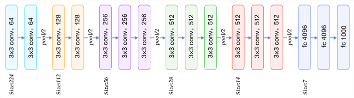
图4 VGG16模型
db_train = tf.data.Dataset.from_tensor_slices((x_train,y_train))
db_train = db_train.shuffle(1000).batch(4)

db_test = tf.data.Dataset.from_tensor_slices((x_test,y_test))

sample = next(iter(db_train))
print("sample: ",sample[0].shape,sample[1].shape)

#--------------------------------卷积神经网络-----------------------------------------
conv_layers = [
    layers.Conv2D(64, kernel_size=[3, 3], padding="same", activation=tf.nn.relu),
    layers.Conv2D(64, kernel_size=[3, 3], padding="same", activation=tf.nn.relu),
    layers.MaxPool2D(pool_size=[4, 4], strides=4, padding='same'),

    # unit 2
    layers.Conv2D(128, kernel_size=[3, 3], padding="same", activation=tf.nn.relu),
    layers.Conv2D(128, kernel_size=[3, 3], padding="same", activation=tf.nn.relu),
    layers.MaxPool2D(pool_size=[4, 4], strides=4, padding='same'),

    # unit 3
    layers.Conv2D(256, kernel_size=[3, 3], padding="same", activation=tf.nn.relu),
    layers.Conv2D(256, kernel_size=[3, 3], padding="same", activation=tf.nn.relu),
    layers.MaxPool2D(pool_size=[4, 4], strides=4, padding='same'),

    # unit 4
    layers.Conv2D(512, kernel_size=[3, 3], padding="same", activation=tf.nn.relu),
    layers.Conv2D(512, kernel_size=[3, 3], padding="same", activation=tf.nn.relu),
    layers.MaxPool2D(pool_size=[2, 2], strides=2, padding='same'),

    # unit 5
    layers.Conv2D(512, kernel_size=[3, 3], padding="same", activation=tf.nn.relu),
    layers.Conv2D(512, kernel_size=[3, 3], padding="same", activation=tf.nn.relu),
    layers.MaxPool2D(pool_size=[2, 2], strides=2, padding='same')
]

def main():
    conv_net = Sequential(conv_layers)
    # 测试输出的图片尺寸
    conv_net.build(input_shape=[None, 128, 128, 3])
    x = tf.random.normal([4, 128, 128, 3])
    out = conv_net(x)
    print(out.shape)

    # 设置全连接层
    fc_net = Sequential([
        layers.Dense(256, activation=tf.nn.relu),
        layers.Dense(128, activation=tf.nn.relu),
        layers.Dense(6, activation=None)
    ])

    conv_net.build(input_shape=[None, 128, 128, 3])
    fc_net.build(input_shape=[None, 512])
    optimizer = optimizers.Adam(lr=0.00001)

    variables = conv_net.trainable_variables + fc_net.trainable_variables

    for epoch in range(50):
        for step,(x,y) in enumerate(db_train):
            with tf.GradientTape() as tape:

                out = conv_net(x)

                out = tf.reshape(out,[-1,512])

                logits = fc_net(out)

                y_hot = tf.one_hot(y,depth=3)
                # 计算loss数值
                loss = tf.losses.categorical_crossentropy(y_hot,logits,from_logits=True)
                loss = tf.reduce_mean(loss)

            grads = tape.gradient(loss,variables)
            optimizer.apply_gradients(zip(grads,variables))

            if step % 20 ==0:
                print(epoch, step, "loss ", float(loss))

        total_num = 0
        totsl_correct = 0
        for x,y in db_test:
            x = tf.expand_dims(x,axis=0)
            # print(x.shape)
            out = conv_net(x)
            out = tf.reshape(out,[-1,512])
            logits = fc_net(out)
            prob = tf.nn.softmax(logits,axis=1)

            pred = tf.argmax(prob,axis=1)
            pred = tf.cast(pred,dtype=tf.int32)

            correct = tf.cast(tf.equal(pred,y),dtype=tf.int32)
            correct = tf.reduce_sum(correct)

            total_num += x.shape[0]
            totsl_correct += int(correct)
        acc = totsl_correct/total_num
        print(epoch, acc)
        conv_net.save('weights/conv.h5')
        fc_net.save('weights/fc.h5')
模型T-SNE动态显示
1.生成图片
SNE即stochastic neighbor embedding,其基本思想为在高维空间相似的数据点,映射到低维空间距离也是相似的。SNE把这种距离关系转换为一种条件概率来表示相似性。
本文主要通过对全连接层的最后一层输出层进行动态可视化。第一步生成每个epoch的Figure,将其保存到指定的文件夹。最后,利用gif工具制作动态显示图片。万变不离其中,方法有很多种,能实现出效果来就是好。
原理参考:t-SNE数据降维(2维3维)及可视化_t-sne降维_小刘同学_的博客-CSDN博客
    #轴承数据训练
    for epoch in range(20):
        # 定义列表,data_xx存放训练数据,data_y存放训练数据标签
        data_xx = []
        data_y = []

        for step,(x,y) in enumerate(db_train):
            with tf.GradientTape() as tape:
                #计算一个batchsize的卷积神经网络输出
                out = conv_net(x)
                #卷积神经网络输出数据进行reshape[-1,512]
                out = tf.reshape(out,[-1,512])
                #reshape的数据输入到全连接层
                logits = fc_net(out)
                #最终输出数据进行one_hot转换
                y_hot = tf.one_hot(y,depth=6)
                # 计算loss数值
                loss = tf.losses.categorical_crossentropy(y_hot,logits,from_logits=True)
                loss = tf.reduce_mean(loss)

            grads = tape.gradient(loss,variables)
            optimizer.apply_gradients(zip(grads,variables))

            #每隔20个bachsize,输出一次loss数值
            if step % 20 ==0:
                print(epoch, step, "loss ", float(loss))

            if epoch >= 2:
                # 列出对应元素的标签值
                data_y.extend(y)
                # 获取所有训练后的样本数据
                for i in range(len(logits)):
                    # 得到训练的样本
                    data_xx.append(logits[i])
                #每次epoch将data_y和data_xx列表转换为numpy数据


        if epoch >= 2:
            data_y = np.array(data_y)
            data_xx = np.array(data_xx)
            # print("data_xx", data_xx.shape)
            # print("data_y", data_y.shape)
            # print("data_y", data_y)
            #进行tsne降维
            tsne = manifold.TSNE(n_components=2, init='pca')
            X_tsne = tsne.fit_transform(data_xx)

            #将降维数据进行可视化显示
            x_min, x_max = X_tsne.min(0), X_tsne.max(0)
            X_norm = (X_tsne - x_min) / (x_max - x_min)  # 归一化

            for i in range(len(X_norm)):
                # plt.text(X_norm[i, 0], X_norm[i, 1], str(y[i]), color=plt.cm.Set1(y[i]),
                if data_y[i] == 0:
                    color = 'r'
                if data_y[i] == 1:
                    color = 'g'
                if data_y[i] == 2:
                    color = 'b'
                if data_y[i] == 3:
                    color = 'c'
                if data_y[i] == 4:
                    color = 'm'
                if data_y[i] == 5:
                    color = 'k'
                #          fontdict={'weight': 'bold', 'size': 9})
                plt.scatter(X_norm[i][0], X_norm[i][1], c=color, cmap=plt.cm.Spectral)

            plt.xticks([])
            plt.yticks([])
            plt.savefig("E:/tsne_figure/" + str(epoch) + ".png")
            plt.close('all')
2.生成gif
# 初始化图片地址文件夹途径

image_path = 'E:/tsne_figure/'

# 获取文件列表

files = os.listdir(image_path)

# 定义第一个文件的全局路径

file_first_path = os.path.join(image_path, files[0])

# 获取Image对象

img = Image.open(file_first_path)

# 初始化文件对象数组

images = []

for image in files[:]:
    # 获取当前图片全量路径

    img_path = os.path.join(image_path, image)

    # 将当前图片使用Image对象打开、然后加入到images数组

    images.append(Image.open(img_path))

# 保存并生成gif动图

img.save('beauty.gif', save_all=True, append_images=images, loop=0, duration=200)
3.效果演示
电脑运算力不行,20个epoch足足跑了一个晚上。最后loss稳定在0.005左右,通过tsne可视化显示,基本实现对不同类型的分离。


 487
487

 被折叠的 条评论
为什么被折叠?
被折叠的 条评论
为什么被折叠?
 到【灌水乐园】发言


