Python 西瓜书编程实现标准BP算法和累积BP算法+loss可视化（可以直接运行）

西瓜数据集3.0
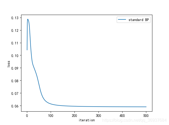
标准BP算法：求单个样本的均方误差（公式5.4）；
参数更新非常频繁;
需要更多次数迭代。（这一点在loss曲线中可以明显看出来）
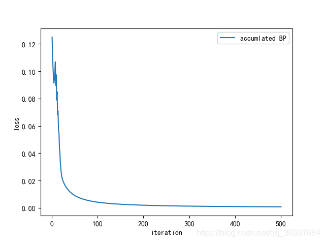
累积BP算法：求所有训练样例的均方误差（公式5.16）；
参数更新频率低得多；
累积误差下降到一定程度之后，进一步下降慢。

# -*- coding: utf-8 -*-
#单隐层网络
import pandas as pd
import numpy as np
from sklearn.preprocessing import LabelEncoder
from sklearn.preprocessing import StandardScaler
import matplotlib.pyplot as plt
seed = 2019
import random
np.random.seed(seed)  # Numpy module.
random.seed(seed)  # Python random module.

plt.rcParams['font.sans-serif'] = ['SimHei'] #用来正常显示中文标签
plt.rcParams['axes.unicode_minus'] = False #用来正常显示负号
plt.close('all')

def preprocess(data):
    #1.将非数映射数字
    for title in data.columns:
        if data[title].dtype=='object':
            encoder = LabelEncoder()
            data[title] = encoder.fit_transform(data[title])         
    #2.去均值和方差归一化
    ss = StandardScaler()
    X = data.drop('好瓜',axis=1)
    Y = data['好瓜']
    X = ss.fit_transform(X)
    x,y = np.array(X),np.array(Y).reshape(Y.shape[0],1)
    return x,y
#定义Sigmoid,求导
def sigmoid(x):
    return 1/(1+np.exp(-x))
def d_sigmoid(x):
    return x*(1-x)

##累积BP算法
def accumulate_BP(x,y,dim=10,eta=0.8,max_iter=500):
    n_samples = x.shape[0]
    w1 = np.zeros((x.shape[1],dim))
    b1 = np.zeros((n_samples,dim))
    w2 = np.zeros((dim,1))
    b2 = np.zeros((n_samples,1))
    losslist = []
    for ite in range(max_iter):
        ##前向传播   
        u1 = np.dot(x,w1)+b1
        out1 = sigmoid(u1)
        u2 = np.dot(out1,w2)+b2
        out2 = sigmoid(u2)
        loss = np.mean(np.square(y - out2))/2
        losslist.append(loss)
        print('iter:%d  loss:%.4f'%(ite,loss))
        ##反向传播
        ##标准BP
        d_out2 = -(y - out2)
        d_u2 = d_out2*d_sigmoid(out2)
        d_w2 = np.dot(np.transpose(out1),d_u2)
        d_b2 = d_u2
        d_out1 = np.dot(d_u2,np.transpose(w2))
        d_u1 = d_out1*d_sigmoid(out1)
        d_w1 = np.dot(np.transpose(x),d_u1)
        d_b1 = d_u1
        ##更新
        w1 = w1 - eta*d_w1
        w2 = w2 - eta*d_w2
        b1 = b1 - eta*d_b1
        b2 = b2 - eta*d_b2
    ##Loss可视化
    plt.figure()
    plt.plot([i+1 for i in range(max_iter)],losslist)
    plt.legend(['accumlated BP'])
    plt.xlabel('iteration')
    plt.ylabel('loss')
    plt.show()
    return w1,w2,b1,b2

##标准BP算法
def standard_BP(x,y,dim=10,eta=0.8,max_iter=500): 
    n_samples = 1
    w1 = np.zeros((x.shape[1],dim))
    b1 = np.zeros((n_samples,dim))
    w2 = np.zeros((dim,1))
    b2 = np.zeros((n_samples,1))
    losslist = []
    for ite in range(max_iter):
        loss_per_ite = []
        for m in range(x.shape[0]):
            xi,yi = x[m,:],y[m,:]
            xi,yi = xi.reshape(1,xi.shape[0]),yi.reshape(1,yi.shape[0])
            ##前向传播   
            u1 = np.dot(xi,w1)+b1
            out1 = sigmoid(u1)
            u2 = np.dot(out1,w2)+b2
            out2 = sigmoid(u2)
            loss = np.square(yi - out2)/2
            loss_per_ite.append(loss)
            print('iter:%d  loss:%.4f'%(ite,loss))
            ##反向传播
            ##标准BP
            d_out2 = -(yi - out2)
            d_u2 = d_out2*d_sigmoid(out2)
            d_w2 = np.dot(np.transpose(out1),d_u2)
            d_b2 = d_u2
            d_out1 = np.dot(d_u2,np.transpose(w2))
            d_u1 = d_out1*d_sigmoid(out1)
            d_w1 = np.dot(np.transpose(xi),d_u1)
            d_b1 = d_u1
            ##更新
            w1 = w1 - eta*d_w1
            w2 = w2 - eta*d_w2
            b1 = b1 - eta*d_b1
            b2 = b2 - eta*d_b2   
        losslist.append(np.mean(loss_per_ite))
    ##Loss可视化
    plt.figure()
    plt.plot([i+1 for i in range(max_iter)],losslist)
    plt.legend(['standard BP'])
    plt.xlabel('iteration')
    plt.ylabel('loss')
    plt.show()
    return w1,w2,b1,b2

def main():
    data = pd.read_table('watermelon30.txt',delimiter=',')
    data.drop('编号',axis=1,inplace=True)
    x,y = preprocess(data)
    dim = 10
#    _,_,_,_ = standard_BP(x,y,dim)
    w1,w2,b1,b2 = accumulate_BP(x,y,dim)
    #测试
    u1 = np.dot(x,w1)+b1
    out1 = sigmoid(u1)
    u2 = np.dot(out1,w2)+b2
    out2 = sigmoid(u2)  
    y_pred = np.round(out2)
    result = pd.DataFrame(np.hstack((y,y_pred)),columns=['真值','预测'] )     
    result.to_excel('result_numpy.xlsx',index=False)

if __name__=='__main__':
    main()