


写在最前
实现平台:MATLAB R2022a
本文仅供学习参考,切忌照搬照抄
觉得有用请点个赞吧🏆
实验一:直线的生成
一、实验内容
根据提供的程序框架,修改部分代码,完成画一条直线的功能(中点画线法,Bresenham画线法,DDA画线法),只要求实现在第一象限内的直线。
二、算法原理介绍
1.DDA画线法
DDA画线法是用于在计算机屏幕上绘制直线的一种基本算法。它基于直线方程 y = mx + c 的概念,其中 m 是斜率,c 是截距。
算法步骤:
1.确定直线的起始点 (x1, y1) 和结束点 (x2, y2);
2.计算直线在 x 和 y 方向上的增量(dx 和 dy);
3.选择增量较大的方向作为步长(steps);
4.计算在步长内 x 和 y 方向上的增量步长(xIncrement 和 yIncrement);
5.从起始点开始,在每个步长上计算像素点坐标并绘制直线;
算法优点:简单易懂;
算法缺点:可能存在精度损失,因为它在每个步长上对坐标进行四舍五入,这可能导致直线的绘制与实际期望有些偏差。
2.Bresenham画线法
Bresenham算法是一种用于在离散坐标系统中绘制直线的算法。它与DDA相似,但是更高效,因为它利用整数运算和位操作来减少计算量。
算法步骤:
1.计算直线两端点的坐标差值的绝对值,即dx和dy;
2.确定步进方向:通过比较起点和终点的x坐标及y坐标来确定步进方向,这决定了x和y每次递增或递减的方式;
3.初始化起始点,开始绘制直线,并绘制起点;
4.根据斜率(dx和dy的比值)的大小,分为两种情况:
a. 如果dx > dy,步进量较大在x方向上,此时以x为基准进行递增或递减,y方向递增或递减的同时,通过一个判别式(p)来决定是否需要更新y值;
b. 如果dy > dx,步进量较大在y方向上,原理与dx > dy相似,只是以y为基准进行递增或递减,x方向递增或递减的同时,通过一个判别式(p)来决定是否需要更新x值;
5.在每一步迭代中,根据判别式(p)的值来决定是否需要更新x或y的值,以在图上绘制出直线上的点;
这个算法的精髓在于,它通过计算判别式(p)的值,避免了使用浮点数运算,而是通过整数运算和位操作来优化直线绘制的过程,从而提高了效率。
3.中点画线法
中点画线法利用一个判别式(p)来确定直线路径上的下一个像素点,从而减少了浮点运算,提高了效率。
算法步骤:
1.计算直线两端点的坐标差值(dx 和 dy)以确定直线在 x 和 y 方向的增量;
2.确定要进行的步数(steps),取 dx 和 dy 中绝对值较大的值;
3.计算 x 和 y 方向的增量;
4.初始化判别式(p),它用于判断下一个点的位置;
5.在循环中,根据判别式的值决定下一个点的位置:如果判别式小于 0,则选择 x 和 y 方向都增量;否则选择 x 和 y 方向同时增量,并更新判别式的值;
6.在每一步迭代中,绘制出直线上的点。
三、程序源代码
1.DDA画线法
function DDA(x1, y1, x2, y2)
    % DDA_Line 函数使用 DDA 算法生成直线
    % 输入参数:
    % x1, y1: 直线起始点坐标
    % x2, y2: 直线结束点坐标

    dx = x2 - x1; % 计算x方向增量
    dy = y2 - y1; % 计算y方向增量

    if abs(dx) >= abs(dy) % 判断斜率绝对值大小,以决定主要步进轴
        steps = abs(dx); % 确定主要步数
    else
        steps = abs(dy);
    end

    xIncrement = dx / steps; % 计算x方向增量
    yIncrement = dy / steps; % 计算y方向增量

    x = x1; % 初始化x坐标
    y = y1; % 初始化y坐标
    plot(round(x), round(y), 'o'); % 绘制起始点

    for k = 1:steps
        x = x + xIncrement; % 更新x坐标
        y = y + yIncrement; % 更新y坐标
        hold on; % 保持图形上的点
        plot(round(x), round(y), 'o'); % 绘制直线上的点
    end
end
2.Bresenham画线法
function Bresenham(x1, y1, x2, y2)
% Bresenham_Line 函数使用 Bresenham 算法生成直线
% 输入参数:
% x1, y1: 直线起始点坐标
% x2, y2: 直线结束点坐标

    dx = abs(x2 - x1); % 计算x方向增量的绝对值
    dy = abs(y2 - y1); % 计算y方向增量的绝对值

    if x1 < x2
        x_increment = 1;
    else
        x_increment = -1;
    end

    if y1 < y2
        y_increment = 1;
    else
        y_increment = -1;
    end

    x = x1; % 初始化x坐标
    y = y1; % 初始化y坐标
    plot(x, y, 'o'); % 绘制起始点

    if dx > dy
        p = 2 * dy - dx;
        for i = 1:dx
            if p >= 0
                y = y + y_increment;
                p = p - 2 * dx;
            end
            x = x + x_increment;
            p = p + 2 * dy;
            hold on; % 保持图形上的点
            plot(x, y, 'o'); % 绘制直线上的点
        end
    else
        p = 2 * dx - dy;
        for i = 1:dy
            if p >= 0
                x = x + x_increment;
                p = p - 2 * dy;
            end
            y = y + y_increment;
            p = p + 2 * dx;
            hold on; % 保持图形上的点
            plot(x, y, 'o'); % 绘制直线上的点
        end
    end
end
3.中点画线法
function Midpoint_Line(x1, y1, x2, y2)
    % Midpoint_Line 函数使用中点画线法生成直线
    % 输入参数:
    %   x1, y1: 直线起始点坐标
    %   x2, y2: 直线结束点坐标

    dx = x2 - x1; % 计算x方向增量
    dy = y2 - y1; % 计算y方向增量

    x = x1; % 初始化x坐标
    y = y1; % 初始化y坐标

    plot(x, y, 'o'); % 绘制起始点

    if abs(dx) > abs(dy)
        steps = abs(dx);
    else
        steps = abs(dy);
    end

    xIncrement = dx / steps; % 计算x方向增量
    yIncrement = dy / steps; % 计算y方向增量

    p = 2 * abs(dy) - abs(dx); % 初始判别式值

    for i = 1:steps
        if p < 0
            x = x + xIncrement; % 更新x坐标
            y = y + yIncrement; % 更新y坐标
            p = p + 2 * abs(dy); % 更新判别式值
        else
            x = x + xIncrement; % 更新x坐标
            y = y + yIncrement; % 更新y坐标
            p = p + 2 * abs(dy) - 2 * abs(dx); % 更新判别式值
        end
        hold on; % 保持图形上的点
        plot(x, y, 'o'); % 绘制直线上的点
    end
end
四、实验结果
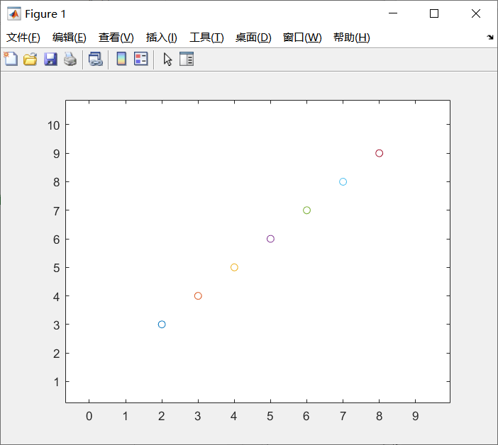
1.DDA画线法
DDA测试案例1:(x1, y1, x2, y2)=(2,3,8,9)
DDA测试案例2:(x1, y1, x2, y2)=(11,4,5,9)

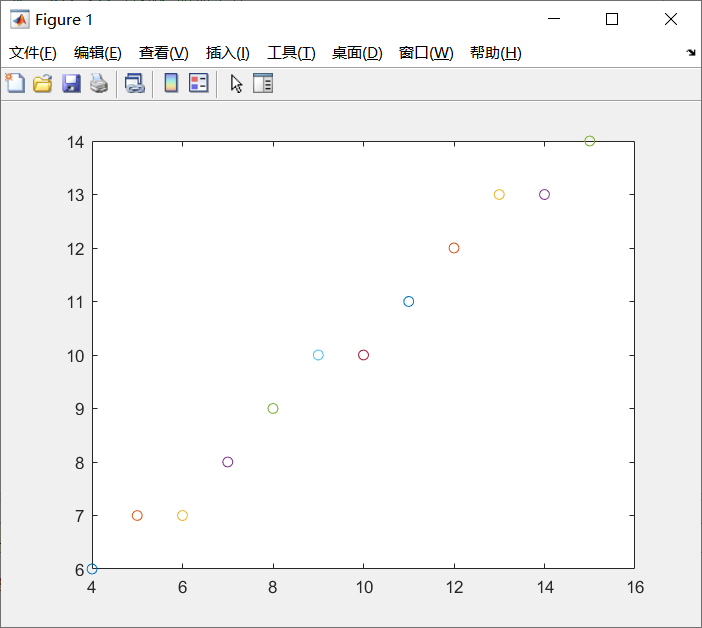
2.Bresenham画线法
测试案例1:(x1, y1, x2, y2)=(4,6,15,14)
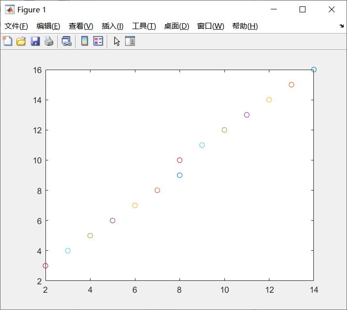
测试案例2:(x1, y1, x2, y2)=(14,16,2,3)
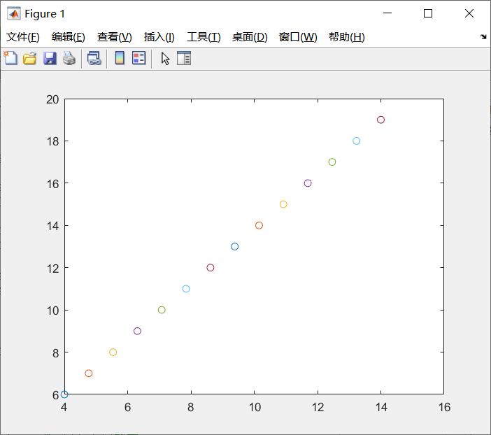
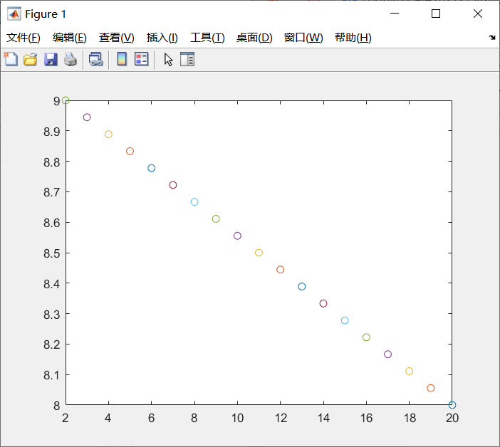
3.中点画线法
测试案例1:(x1, y1, x2, y2)=(4,6,14,19)
测试案例2:(x1, y1, x2, y2)=(20,8,2,9)
实验二:用扫描线算法实现多边形填充
一、实验内容
用水平扫描线从上到下扫描由点线段构成的多段定义的多边形。
二、算法原理介绍
扫描线算法是一种用于多边形填充的基于扫描线的方法。其原理是利用扫描线从多边形的最低点向上扫描,找到多边形边界与扫描线的交点,然后对这些交点之间的区域进行填充。
算法步骤如下:
1.建立边表:遍历多边形的每条边,对于每条边,计算其与扫描线的交点并记录下来。这些边被存储在边表中,其中每个条目对应扫描线的一个位置;
2.扫描线循环:从多边形最低点开始向上扫描线。对于每条扫描线,将与该扫描线有交点的边添加到活性边表中。活性边表存储当前扫描线上的边,即这些边与扫描线相交但尚未处理的边;
3.活性边表的维护:随着扫描线的上升,需要更新活性边表。移除不再与扫描线相交的边,同时根据交点的 x 坐标对活性边进行排序;
4.填充区域:对于每对交点之间的区域,使用填充算法(例如,从左到右的像素填充或其他方法),填充多边形内部;
5.更新边表:随着扫描线的移动,更新活性边表中边的 x 坐标值。这些坐标值是在 x 轴上与扫描线相交的下一个点;
6.重复扫描线直到完成:持续扫描线直到达到多边形的最高点。
三、程序源代码
function scanline_fill(vertices)
    % 计算多边形的顶点数量
    num_vertices = size(vertices, 1);
    % 获取最小和最大 Y 坐标以确定扫描线的范围
    min_y = min(vertices(:, 2));
    max_y = max(vertices(:, 2));

    % 创建边表和活性边表
    edge_table = cell(1, max_y - min_y + 1);
    active_edge_table = [];

    % 填充边表
    for i = 1:num_vertices
        start_point = vertices(i, :);
        end_point = vertices(mod(i, num_vertices) + 1, :);

        if start_point(2) ~= end_point(2)
            % 计算边的斜率倒数
            edge = struct(...
                'y_max', max(start_point(2), end_point(2)), ...
                'x_min', min(start_point(1), end_point(1)), ...
                'slope_inv', (end_point(1) - start_point(1)) / (end_point(2) - start_point(2)), ...
                'is_processed', false ...
            );

            % 将边加入边表对应的位置
            y = min(start_point(2), end_point(2)) - min_y + 1;
            if isempty(edge_table{y})
                edge_table{y} = edge;
            else
                edge_table{y} = [edge_table{y}, edge];
            end
        end
    end

    % 开始绘图
    hold on;

    % 绘制多边形的边线
    for i = 1:num_vertices
        start_point = vertices(i, :);
        end_point = vertices(mod(i, num_vertices) + 1, :);
        plot([start_point(1), end_point(1)], [start_point(2), end_point(2)], 'b');
    end

    % 扫描线算法循环
    for y = 1:(max_y - min_y + 1)
        % 将新的边从边表添加到活性边表
        if ~isempty(edge_table{y})
            active_edge_table = [active_edge_table, edge_table{y}];
        end

        % 移除不再可见的边
        active_edge_table = active_edge_table([active_edge_table.y_max] > y + min_y - 1);

        % 根据 x_min 排序活性边表
        [~, sort_index] = sort([active_edge_table.x_min]);
        active_edge_table = active_edge_table(sort_index);

        % 填充当前扫描线的像素
        for i = 1:2:numel(active_edge_table)
            for x = ceil(active_edge_table(i).x_min):floor(active_edge_table(i + 1).x_min)
                plot(x, y + min_y - 1, 'r.');
            end
        end

        % 更新 x_min
        for i = 1:numel(active_edge_table)
            active_edge_table(i).x_min = active_edge_table(i).x_min + active_edge_table(i).slope_inv;
        end
    end

    % 结束绘图
    hold off;
end
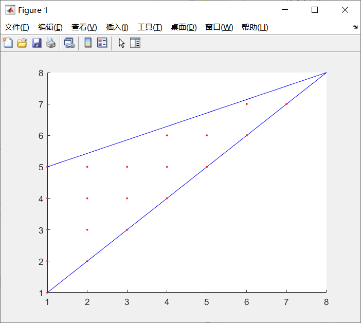
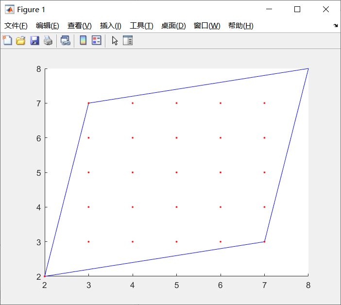
四、实验结果
测试案例1:vertices=[1,1;1,5;8,8]
测试案例2:vertices=[2,2;3,7;8,8;7,3]
实验三:用Cohen-Sutherland裁剪算法实现直线段裁剪
一、实验内容
用Cohen-Sutherland裁剪算法实现直线段裁剪。
二、算法原理介绍
Cohen-Sutherland裁剪算法是一种用于线段裁剪的基本方法,它通过利用区域编码来判断线段与裁剪窗口之间的相对位置关系,并进行相应的裁剪。
算法步骤:
1.区域编码
裁剪窗口被分成九个区域:内部和外部,以及左、右、上、下、左上、右上、左下和右下。每个点都根据其位置被分配一个区域编码,根据其相对于裁剪窗口的位置关系,编码是一个4位二进制数;
2.算法流程
线段的两个端点被分别编码。检查这两个端点的区域编码,如果它们都在裁剪窗口内部,则该线段完全可见,被接受;如果两个端点都在窗口的同一边界之外,那么整个线段都在一个界限之外,被拒绝;如果端点在不同的区域,则需要计算交点,更新端点,继续检查直到该线段完全在裁剪窗口内部或完全在窗口外部;
3.裁剪
当线段跨越窗口边界时,找到与窗口边界的交点;通过计算直线与边界的交点来更新线段端点,使得线段在窗口内部或者与窗口边界相交;
4.重复迭代
更新线段端点的位置,重新计算区域编码,直到线段完全在窗口内部、完全在窗口外部或不再与窗口相交;
5.接受或拒绝
如果线段完全在窗口内部,则被接受,绘制剪裁后的线段;如果线段完全在窗口外部,则被拒绝,不进行绘制;
这个算法的主要优点是简单直观,效率高;
缺点是不适合于多边形裁剪,且裁剪时可能需要多次计算交点,计算成本高。
三、程序源代码
function cohenSutherlandClip(x1, y1, x2, y2, xmin, ymin, xmax, ymax)
    % 设置区域代码
    INSIDE = 0; % 0000
    LEFT = 1;   % 0001
    RIGHT = 2;  % 0010
    BOTTOM = 4; % 0100
    TOP = 8;    % 1000

    % 计算区域代码
    function code = computeCode(x, y)
        code = INSIDE; % 初始设为内部点
        if x < xmin % 超出左边界
            code = code | LEFT;
        elseif x > xmax % 超出右边界
            code = code | RIGHT;
        end
        if y < ymin % 超出下边界
            code = code | BOTTOM;
        elseif y > ymax % 超出上边界
            code = code | TOP;
        end
    end

    % 计算初始点的区域代码
    code1 = computeCode(x1, y1);
    code2 = computeCode(x2, y2);

    accept = false; % 是否接受直线段

    while true
        if bitand(code1, code2) ~= 0 % 完全在某一侧
            break;
        elseif bitor(code1, code2) == 0 % 完全在内部
            accept = true;
            break;
        else
            x = 0;
            y = 0;
            code = code1;

            if code == INSIDE % 在内部,选择另一个点
                code = code2;
            end

            % 计算交点坐标
            if bitand(code, TOP) % 与上边界相交
                x = x1 + (x2 - x1) * (ymax - y1) / (y2 - y1);
                y = ymax;
            elseif bitand(code, BOTTOM) % 与下边界相交
                x = x1 + (x2 - x1) * (ymin - y1) / (y2 - y1);
                y = ymin;
            elseif bitand(code, RIGHT) % 与右边界相交
                y = y1 + (y2 - y1) * (xmax - x1) / (x2 - x1);
                x = xmax;
            elseif bitand(code, LEFT) % 与左边界相交
                y = y1 + (y2 - y1) * (xmin - x1) / (x2 - x1);
                x = xmin;
            end

            if code == code1 % 更新第一个点的坐标和区域代码
                x1 = x;
                y1 = y;
                code1 = computeCode(x1, y1);
            else % 更新第二个点的坐标和区域代码
                x2 = x;
                y2 = y;
                code2 = computeCode(x2, y2);
            end
        end
    end

    if accept
        fprintf('线段被接受: (%d, %d) to (%d, %d)\n', x1, y1, x2, y2);
        plot([x1, x2], [y1, y2], 'r', 'LineWidth', 2); % 绘制裁剪后的直线段
    else
        fprintf('线段被拒绝\n');
    end
    hold on;
    plot([xmin, xmin, xmax, xmax, xmin], [ymin, ymax, ymax, ymin, ymin], 'k--', 'LineWidth', 1.5); % 绘制裁剪窗口
    axis([xmin-10 xmax+10 ymin-10 ymax+10]); % 设置坐标轴范围
    grid on;
    xlabel('X轴');
    ylabel('Y轴');
    title('Cohen-Sutherland裁剪算法');
end
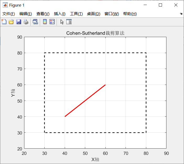
四、实验结果
测试案例1:
(x1, y1, x2, y2, xmin, ymin, xmax, ymax)=(40,40,60,60,30,30,80,80)
在这种情况下,两个端点都在窗口中,线段被完全接受,不会裁剪

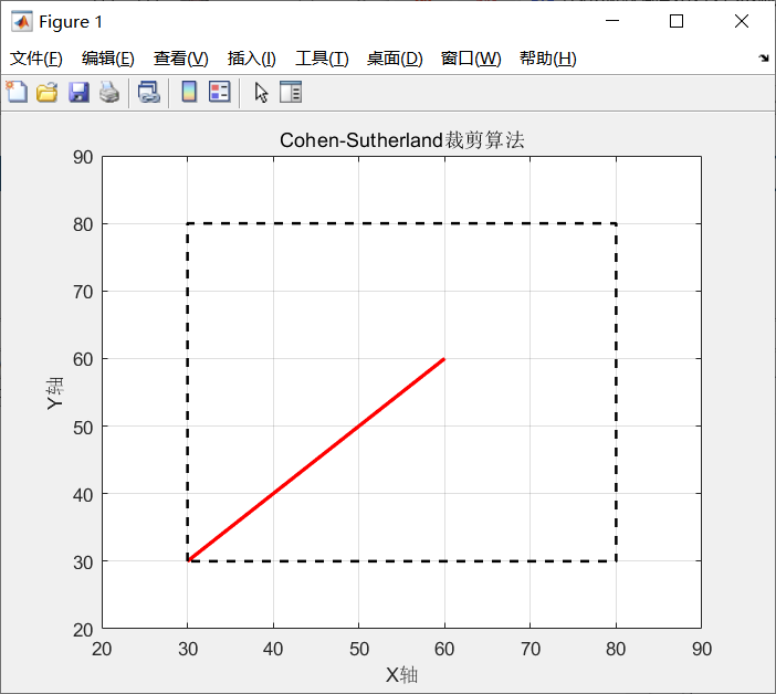
测试案例2:
(x1, y1, x2, y2, xmin, ymin, xmax, ymax)=(20,20,60,60,30,30,80,80)
在这种情况下,第一个点不在窗口中,第二个点在窗口中,线段被接受一部分,发生了裁剪

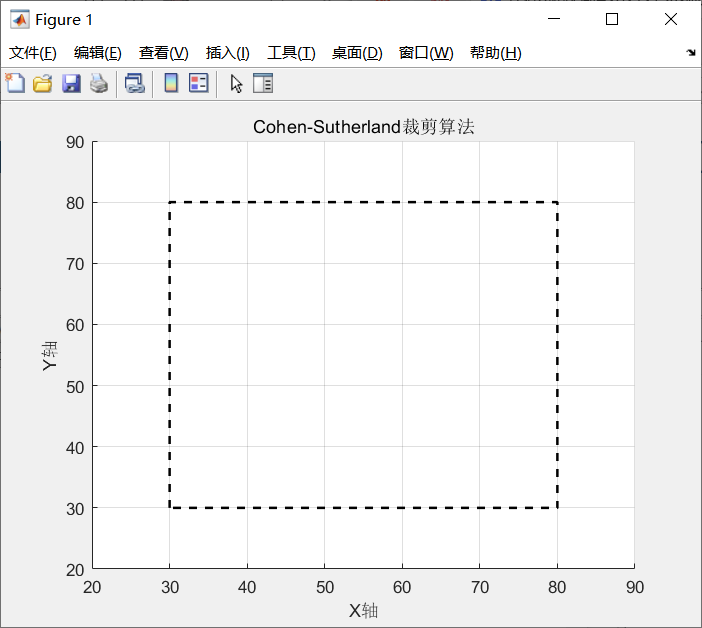
测试案例3:
(x1, y1, x2, y2, xmin, ymin, xmax, ymax)=(20,20,80,20,30,30,80,80)
在这种情况下,两个点都在窗口外,线段被拒绝

实验四:二维图形的缩放、旋转,平移,组合变换和对称变换
一、实验内容
完成二维图形的缩放、旋转,平移,组合变换以及对称变换。
二、算法原理介绍
**实现平台:**MATLAB R2022a
1.二维图形的缩放
二维图形缩放需要通过缩放矩阵将二位图形的对应点按比例进行缩放,最后重新绘制图形。
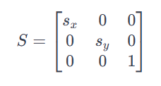
缩放矩阵通常是一个 2x2 的矩阵,其一般形式如下:
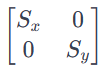
这里的Sx和Sy分别代表了在水平和垂直方向上的缩放因子。如果 Sx和Sy的值大于 1,则会产生放大效果;若小于 1,则会产生缩小效果;若等于 1,则表示不发生变化。
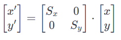
对于任意的点或向量(x,y),应用缩放矩阵后可以得到缩放后的点或向量(x’,y’),其计算方式为:
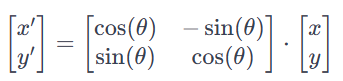
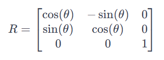
2.二维图形的旋转
实现二维图形旋转需要考虑旋转矩阵。矩阵如下:
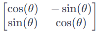
对于任意的点或向量(x,y),应用旋转矩阵后可以得到缩放后的点或向量(x’,y’),其计算方式为:
以一个矩形为例,旋转步骤为:
1.构建矩形的顶点坐标;
2.计算矩形的中心坐标;
3.将矩形的顶点坐标移到原点;
4.计算旋转矩阵;
5.组合顶点坐标矩阵;
6.应用旋转矩阵到矩形的每个顶点上;
7.将旋转后的矩形顶点坐标移回原来的位置;
8.绘制原始矩形和旋转后的矩形。
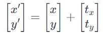
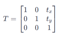
3.二维图形的平移
平移可以用平移向量矩阵表示。平移矩阵如下:

对于任意的点或向量(x,y),应用平移矩阵后可以得到缩放后的点或向量(x’,y’),其计算方式为:
4.二维图形的组合变换
当需要进行多个变换(如平移、旋转、缩放等)时,可以将这些变换表示为矩阵,并将它们按顺序相乘得到一个组合变换矩阵,然后将这个矩阵应用于原始图形的顶点来实现组合变换。
变换过程如下:
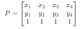
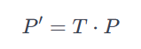
1.平移矩阵
2.矩形顶点矩阵
3.将矩形顶点坐标移动到原点
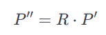
4.旋转矩阵
5.旋转后的矩形顶点矩阵
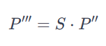
6.缩放矩阵
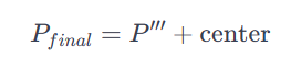
7.最终变换矩阵
8.将顶点坐标移回原位置
5.二维图形的对称变换
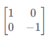
需要构建相应的对称变换矩阵。这里我选择实现关于x轴对称,关于y轴对称和关于原点对称三种情况。对应的矩阵如下:
关于x轴对称:
关于y轴对称:

关于原点对称:
三、程序源代码
1.二维图形的缩放(以矩形为例)
function Scaled_Rectangle(bottom_left_x, bottom_left_y, top_right_x, top_right_y, sx, sy)
    % Scaled_Rectangle 函数用于对矩形进行缩放
    % 输入参数:
    %   bottom_left_x, bottom_left_y: 矩形左下角坐标
    %   top_right_x, top_right_y: 矩形右上角坐标
    %   sx, sy: 水平和垂直方向的缩放因子

    % 应用缩放矩阵到矩形的每个顶点上
    bottom_left_scaled_x = bottom_left_x * sx;
    bottom_left_scaled_y = bottom_left_y * sy;
    top_right_scaled_x = top_right_x * sx;
    top_right_scaled_y = top_right_y * sy;

    % 绘制原始矩形
    plot([bottom_left_x, top_right_x, top_right_x, bottom_left_x, bottom_left_x], [bottom_left_y, bottom_left_y, top_right_y, top_right_y, bottom_left_y], '-o', 'DisplayName', 'Original Rectangle');
    hold on;

    % 绘制缩放后的矩形
    plot([bottom_left_scaled_x, top_right_scaled_x, top_right_scaled_x, bottom_left_scaled_x, bottom_left_scaled_x], [bottom_left_scaled_y, bottom_left_scaled_y, top_right_scaled_y, top_right_scaled_y, bottom_left_scaled_y], '-o', 'DisplayName', 'Scaled Rectangle');

    xlabel('X-axis');
    ylabel('Y-axis');
    title('Scaling of Rectangle');
    legend;
end
2.二维图形的旋转
function Rotated_Rectangle(bottom_left_x, bottom_left_y, top_right_x, top_right_y, theta)
    % Rotated_Rectangle 函数用于对矩形进行旋转
    % 输入参数:
    %   bottom_left_x, bottom_left_y: 矩形左下角坐标
    %   top_right_x, top_right_y: 矩形右上角坐标
    %   theta: 旋转角度(弧度)

    % 构建矩形的顶点坐标
    x = [bottom_left_x, top_right_x, top_right_x, bottom_left_x, bottom_left_x];
    y = [bottom_left_y, bottom_left_y, top_right_y, top_right_y, bottom_left_y];

    % 计算矩形的中心坐标
    center_x = (bottom_left_x + top_right_x) / 2;
    center_y = (bottom_left_y + top_right_y) / 2;

    % 将矩形的顶点坐标移到原点
    x = x - center_x;
    y = y - center_y;

    % 计算旋转矩阵
    rotation_matrix = [cos(theta), -sin(theta); sin(theta), cos(theta)];

    % 组合矩形顶点坐标矩阵
    points = [x; y];

    % 应用旋转矩阵到矩形的每个顶点上
    rotated_points = rotation_matrix * points;

    % 将旋转后的矩形顶点坐标移到原来的位置
    rotated_points(1, :) = rotated_points(1, :) + center_x;
    rotated_points(2, :) = rotated_points(2, :) + center_y;

    % 绘制原始矩形(实线)
    plot(x + center_x, y + center_y, '-o', 'DisplayName', 'Original Rectangle');
    hold on;

    % 绘制旋转后的矩形(虚线)
    plot(rotated_points(1, :), rotated_points(2, :), '--o', 'DisplayName', 'Rotated Rectangle');

    xlabel('X-axis');
    ylabel('Y-axis');
    title('Rotation of Rectangle');
    legend;
end
3.二维图形的平移
function Translated_Rectangle(bottom_left_x, bottom_left_y, top_right_x, top_right_y, tx, ty)
    % Translated_Rectangle 函数用于对矩形进行平移
    % 输入参数:
    %   bottom_left_x, bottom_left_y: 矩形左下角坐标
    %   top_right_x, top_right_y: 矩形右上角坐标
    %   tx, ty: 平移向量

    % 构建矩形的顶点坐标
    x = [bottom_left_x, top_right_x, top_right_x, bottom_left_x, bottom_left_x];
    y = [bottom_left_y, bottom_left_y, top_right_y, top_right_y, bottom_left_y];

    % 将矩形的所有顶点坐标按照平移向量进行平移
    x_translated = x + tx;
    y_translated = y + ty;

    % 绘制原始矩形(实线)
    plot([x(1), x(2), x(3), x(4), x(1)], [y(1), y(2), y(3), y(4), y(1)], '-o', 'DisplayName', 'Original Rectangle', 'LineWidth', 1.5);
    hold on;

    % 绘制平移后的矩形(虚线)
    plot([x_translated(1), x_translated(2), x_translated(3), x_translated(4), x_translated(1)], [y_translated(1), y_translated(2), y_translated(3), y_translated(4), y_translated(1)], '--o', 'DisplayName', 'Translated Rectangle', 'LineWidth', 1.5);

    xlabel('X-axis');
    ylabel('Y-axis');
    title('Translation of Rectangle');
    legend;
end
4.二维图形的组合变换
function Combined_Transformation_Rectangle(bottom_left_x, bottom_left_y, top_right_x, top_right_y, tx, ty, theta, sx, sy)
    % Combined_Transformation_Rectangle 函数用于对矩形进行组合变换
    % 输入参数:
    %   bottom_left_x, bottom_left_y: 矩形左下角坐标
    %   top_right_x, top_right_y: 矩形右上角坐标
    %   tx, ty: 平移向量
    %   theta: 旋转角度(弧度)
    %   sx, sy: 缩放因子

    % 构建矩形的顶点坐标
    x = [bottom_left_x, top_right_x, top_right_x, bottom_left_x, bottom_left_x];
    y = [bottom_left_y, bottom_left_y, top_right_y, top_right_y, bottom_left_y];

    % 将矩形的所有顶点坐标按照平移向量进行平移
    x_translated = x + tx;
    y_translated = y + ty;

    % 计算矩形的中心坐标
    center_x = (bottom_left_x + top_right_x) / 2;
    center_y = (bottom_left_y + top_right_y) / 2;

    % 将矩形的顶点坐标移到原点
    x_centered = x_translated - center_x;
    y_centered = y_translated - center_y;

    % 计算旋转矩阵
    rotation_matrix = [cos(theta), -sin(theta); sin(theta), cos(theta)];

    % 应用旋转矩阵到矩形的每个顶点上
    rotated_points = rotation_matrix * [x_centered; y_centered];

    % 计算缩放矩阵
    scaling_matrix = [sx, 0; 0, sy];

    % 应用缩放矩阵到矩形的每个顶点上
    scaled_points = scaling_matrix * rotated_points;

    % 将旋转后并且缩放后的矩形顶点坐标移到原来的位置
    scaled_points(1, :) = scaled_points(1, :) + center_x;
    scaled_points(2, :) = scaled_points(2, :) + center_y;

    % 绘制原始矩形(实线)
    plot([x(1), x(2), x(3), x(4), x(1)], [y(1), y(2), y(3), y(4), y(1)], '-o', 'DisplayName', 'Original Rectangle', 'LineWidth', 1.5);
    hold on;

    % 绘制变换后的矩形(虚线)
    plot([scaled_points(1, 1), scaled_points(1, 2), scaled_points(1, 3), scaled_points(1, 4), scaled_points(1, 1)], [scaled_points(2, 1), scaled_points(2, 2), scaled_points(2, 3), scaled_points(2, 4), scaled_points(2, 1)], '--o', 'DisplayName', 'Transformed Rectangle', 'LineWidth', 1.5);

    xlabel('X-axis');
    ylabel('Y-axis');
    title('Combined Transformation of Rectangle');
    legend;
end
5.二维图形的对称变换
function Symmetric_Transformation_Rectangle(bottom_left_x, bottom_left_y, top_right_x, top_right_y)
    % Symmetric_Transformation_Rectangle 函数用于对矩形进行三种对称变换
    % 输入参数:
    %   bottom_left_x, bottom_left_y: 矩形左下角坐标
    %   top_right_x, top_right_y: 矩形右上角坐标

    % 构建矩形的顶点坐标
    x = [bottom_left_x, top_right_x, top_right_x, bottom_left_x, bottom_left_x];
    y = [bottom_left_y, bottom_left_y, top_right_y, top_right_y, bottom_left_y];

    % 绘制原始矩形(实线)
    plot([x(1), x(2), x(3), x(4), x(1)], [y(1), y(2), y(3), y(4), y(1)], '-o', 'DisplayName', 'Original Rectangle', 'LineWidth', 1.5);
    hold on;

    % 构建对称变换矩阵
    x_axis_symmetric_matrix = [1, 0; 0, -1];
    y_axis_symmetric_matrix = [-1, 0; 0, 1];
    origin_symmetric_matrix = [-1, 0; 0, -1];

    % 将矩形的顶点坐标按照对称矩阵进行变换

    % X轴对称变换
    x_axis_transformed_points = x_axis_symmetric_matrix * [x; y];
    % 绘制关于 X 轴对称变换后的矩形(虚线)
    plot([x_axis_transformed_points(1, 1), x_axis_transformed_points(1, 2), x_axis_transformed_points(1, 3), x_axis_transformed_points(1, 4), x_axis_transformed_points(1, 1)], [x_axis_transformed_points(2, 1), x_axis_transformed_points(2, 2), x_axis_transformed_points(2, 3), x_axis_transformed_points(2, 4), x_axis_transformed_points(2, 1)], '--o', 'DisplayName', 'X-axis Symmetric Rectangle', 'LineWidth', 1.5);

    % Y轴对称变换
    y_axis_transformed_points = y_axis_symmetric_matrix * [x; y];
    % 绘制关于 Y 轴对称变换后的矩形(虚线)
    plot([y_axis_transformed_points(1, 1), y_axis_transformed_points(1, 2), y_axis_transformed_points(1, 3), y_axis_transformed_points(1, 4), y_axis_transformed_points(1, 1)], [y_axis_transformed_points(2, 1), y_axis_transformed_points(2, 2), y_axis_transformed_points(2, 3), y_axis_transformed_points(2, 4), y_axis_transformed_points(2, 1)], '--o', 'DisplayName', 'Y-axis Symmetric Rectangle', 'LineWidth', 1.5);

    % 原点对称变换
    origin_transformed_points = origin_symmetric_matrix * [x; y];
    % 绘制关于原点对称变换后的矩形(虚线)
    plot([origin_transformed_points(1, 1), origin_transformed_points(1, 2), origin_transformed_points(1, 3), origin_transformed_points(1, 4), origin_transformed_points(1, 1)], [origin_transformed_points(2, 1), origin_transformed_points(2, 2), origin_transformed_points(2, 3), origin_transformed_points(2, 4), origin_transformed_points(2, 1)], '--o', 'DisplayName', 'Origin Symmetric Rectangle', 'LineWidth', 1.5);

    xlabel('X-axis');
    ylabel('Y-axis');
    title('Symmetric Transformations of Rectangle');
    legend;
end
四、实验结果
1.二维图形的缩放
测试案例1:
(bottom_left_x, bottom_left_y, top_right_x, top_right_y, sx, sy)=(1,1,5,5,2,7)
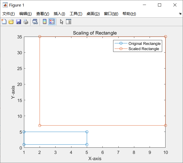
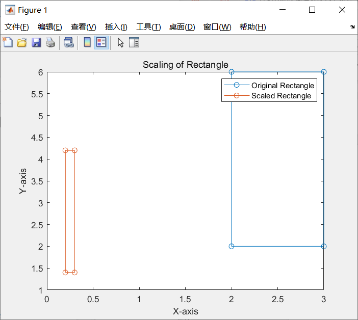
测试案例2:
(bottom_left_x, bottom_left_y, top_right_x, top_right_y, sx, sy)=(2,2,3,6,0.1,0.7)
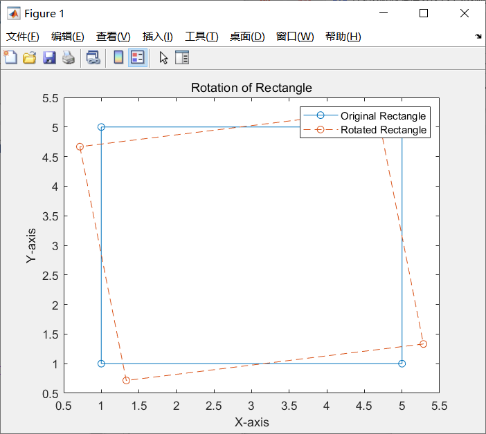
2.二维图形的旋转
测试案例1:
(bottom_left_x, bottom_left_y, top_right_x, top_right_y, theta)=(1,1,5,5,30)
测试案例2:
(bottom_left_x, bottom_left_y, top_right_x, top_right_y, theta)=(2,2,8,8,-75)

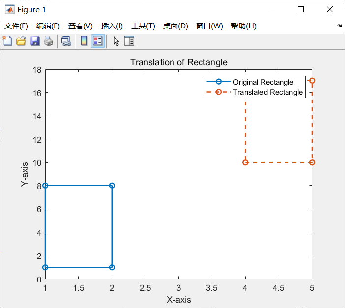
3.二维图形的平移
测试案例1:
(bottom_left_x, bottom_left_y, top_right_x, top_right_y, tx, ty)=(1,1,2,8,3,9)
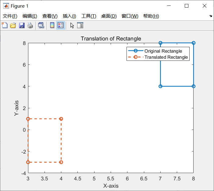
测试案例2:
(bottom_left_x, bottom_left_y, top_right_x, top_right_y, tx, ty)=(8,8,7,4,-4,-7)
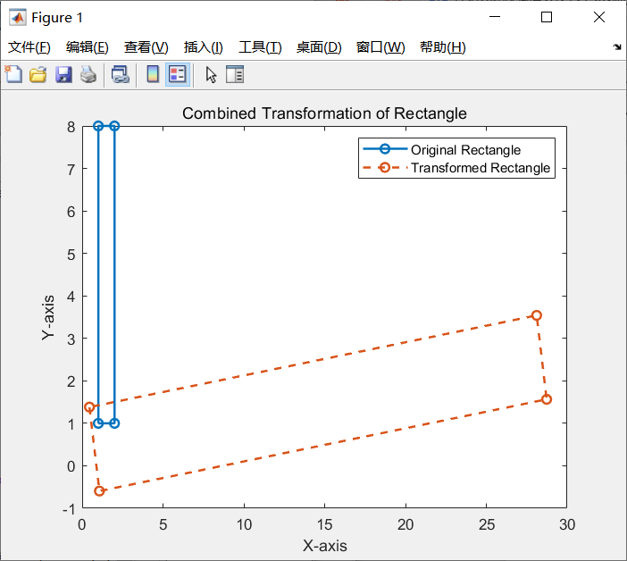
4.二维图形的组合变换
测试案例1:
(bottom_left_x, bottom_left_y, top_right_x, top_right_y, tx, ty, theta, sx, sy)
=(1,1,2,8,2,3,30,4,2)
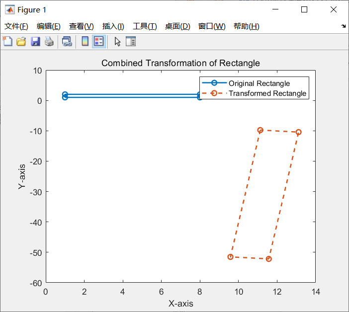
测试案例2:
(bottom_left_x, bottom_left_y, top_right_x, top_right_y, tx, ty, theta, sx, sy)
=(1,1,8,2,5,4,80,2,6)
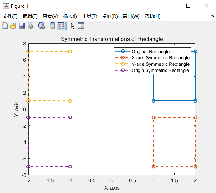
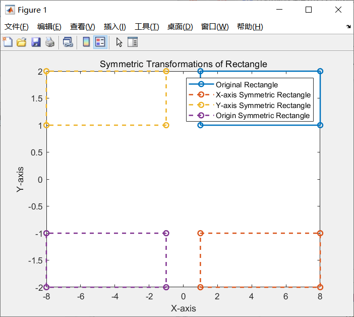
5.二维图形的对称变换
测试案例1:
(bottom_left_x, bottom_left_y, top_right_x, top_right_y)=(1,1,2,7)
测试案例2:
(bottom_left_x, bottom_left_y, top_right_x, top_right_y)=(1,1,8,2)


 2655
2655

 被折叠的 条评论
为什么被折叠?
被折叠的 条评论
为什么被折叠?
 到【灌水乐园】发言


