


 本文深入解析ORB-SLAM2中单应矩阵和基础矩阵的理论与源码实现,阐述如何从这两种矩阵中分解出相机位姿和三维空间点坐标,包括RANSAC算法、阈值选择、模型选择策略等关键步骤。

ORB-SLAM2目录:
一步步带你看懂orbslam2源码–总体框架(一)
一步步带你看懂orbslam2源码–orb特征点提取(二)
一步步带你看懂orbslam2源码–单目初始化(三)
一步步带你看懂orbslam2源码–单应矩阵/基础矩阵,求解R,t(四)
一步步带你看懂orbslam2源码–单目初始化(五)
回顾:
上一节我们主要讲解了对极约束的原理以及F矩阵的求解,单应矩阵的原理以及单应矩阵的求解,RANSAC随机采样一致性算法,阈值选择原理,score计算方式,模型选择策略,并且对创建Frame剩余的部分源码进行补充说明.本章节主要将讲解如何从单应矩阵和基础矩阵中分解出相机位姿和三维空间点坐标,这一部分东北大学的吴博在"ORB-SLAM代码详细解读"PPT中已经进行了详细推导,笔者这次的主要目的是根据吴博的推导过程再讲解一遍,并且完善其中的计算过程,最后还给出了其在orbslam2源码中的实现方式.
理论环节
由上一讲中,我们已经知道单应矩阵
H
H
H的形式:
p
2
=
H
21
p
1
=
K
(
R
+
t
n
T
d
)
K
−
1
p
1
(1)
\begin{aligned} p_2&=H_{21}p_1\\ &=K(R+\frac{tn^T}{d})K^{-1}p_1 \end{aligned}\tag{1}
p2=H21p1=K(R+dtnT)K−1p1(1)
问题转换为:我们如何从
H
21
H_{21}
H21中分解出
R
R
R和
t
t
t,这也是本章节的主要内容,可以将式(1)做进一步变换:
K
−
1
H
21
K
=
R
+
t
n
T
d
(2)
\begin{aligned} K^{-1}H_{21}K& &=R+\frac{tn^T}{d} \end{aligned}\tag{2}
K−1H21K=R+dtnT(2)
令
A
=
d
R
+
t
n
T
A=dR+tn^T
A=dR+tnT,对
A
A
A进行奇异值分解:
A
=
U
Λ
V
T
A=U\Lambda V^T
A=UΛVT,则
Λ
=
U
T
A
V
=
d
U
T
R
V
+
(
U
T
t
)
(
V
T
n
)
T
(3)
\Lambda =U^TAV=dU^TRV+(U^Tt)(V^Tn)^T\tag{3}
Λ=UTAV=dUTRV+(UTt)(VTn)T(3)
因为
U
U
U和
V
V
V为单位正交矩阵,所以考虑
s
=
d
e
t
U
d
e
t
V
,
s
2
=
1
s=detUdetV,s^2=1
s=detUdetV,s2=1
将式(3)变换为:
Λ
=
s
2
d
U
T
R
V
+
(
U
T
t
)
(
V
T
n
)
T
=
(
s
d
)
(
s
U
T
R
V
)
+
(
U
T
t
)
(
V
T
n
)
T
(4)
\Lambda =s^2dU^TRV+(U^Tt)(V^Tn)^T=(sd)(sU^TRV)+(U^Tt)(V^Tn)^T\tag{4}
Λ=s2dUTRV+(UTt)(VTn)T=(sd)(sUTRV)+(UTt)(VTn)T(4)
令
R
′
=
s
U
T
R
V
,
t
′
=
U
T
t
,
n
′
=
V
T
n
,
d
′
=
s
d
R^{'}=sU^TRV,t^{'}=U^Tt,n^{'}=V^Tn,d^{'}=sd
R′=sUTRV,t′=UTt,n′=VTn,d′=sd
则式(4)变为:
Λ
=
d
′
R
′
+
t
′
n
′
T
(5)
\Lambda =d^{'}R^{'}+t^{'}n^{'T}\tag{5}
Λ=d′R′+t′n′T(5)
于是,原问题转换为:如何从式子(5)中的
Λ
\Lambda
Λ分解出
R
′
R^{'}
R′和
t
′
t^{'}
t′,从而可以得到:
{
R
=
1
s
U
R
′
V
T
t
=
U
t
′
(6)
\left\{\begin{aligned} R&=\frac{1}{s}UR^{'}V^T\\ t&=Ut^{'} \end{aligned}\right.\tag{6}
⎩⎨⎧Rt=s1UR′VT=Ut′(6)
注意
s
=
±
1
s=±1
s=±1,这是正交矩阵的性质,引入
s
s
s是为了说明
R
′
R^{'}
R′与
R
R
R,
d
′
d^{'}
d′与
d
d
d存在符号取反的可能. 进一步的:
Λ
=
[
d
1
0
0
0
d
2
0
0
0
d
3
]
=
d
′
R
′
+
t
′
n
′
T
(7)
\Lambda = \begin{bmatrix} d_1 &0 &0\\ 0 &d_2 & 0\\ 0 &0 &d_3 \end{bmatrix}=d^{'}R^{'}+t^{'}n^{'T}\tag{7}
Λ=⎣⎡d1000d2000d3⎦⎤=d′R′+t′n′T(7)
取:
e
1
=
[
1
0
0
]
,
e
2
=
[
0
1
0
]
,
e
3
=
[
0
0
1
]
e_1=\begin{bmatrix} 1\\0\\0 \end{bmatrix}, e_2=\begin{bmatrix} 0\\1\\0 \end{bmatrix}, e_3=\begin{bmatrix} 0\\0\\1 \end{bmatrix}
e1=⎣⎡100⎦⎤,e2=⎣⎡010⎦⎤,e3=⎣⎡001⎦⎤
则:
n
′
=
e
1
=
[
x
1
0
0
]
+
[
0
x
2
0
]
+
[
0
0
x
3
]
=
x
1
e
1
+
x
2
e
2
+
x
3
e
3
(8)
n^{'}= e_1=\begin{bmatrix} x_1\\0\\0 \end{bmatrix}+ \begin{bmatrix} 0\\x_2\\0 \end{bmatrix}+ \begin{bmatrix} 0\\0\\x_3 \end{bmatrix}= x_1e_1+x_2e_2+x_3e_3\tag{8}
n′=e1=⎣⎡x100⎦⎤+⎣⎡0x20⎦⎤+⎣⎡00x3⎦⎤=x1e1+x2e2+x3e3(8)
注意到,由于
n
′
n^{'}
n′是平面的单位法向量,所以
x
1
2
+
x
2
2
+
x
3
2
=
1
x_1^2+x_2^2+x_3^2=1
x12+x22+x32=1
所以式(7)变为:
[
d
1
e
1
d
2
e
2
d
3
e
3
]
=
[
d
′
R
′
e
1
d
′
R
′
e
2
d
′
R
′
e
3
]
+
[
t
′
x
1
t
′
x
2
t
′
x
2
]
(9)
\begin{bmatrix} d_1e_1 & d_2e_2 &d_3e_3 \end{bmatrix}= \begin{bmatrix} d^{'}R^{'}e_1 & d^{'}R^{'}e_2 &d^{'}R^{'}e_3 \end{bmatrix}+ \begin{bmatrix} t^{'}x_1 & t^{'}x_2 &t^{'}x_2 \end{bmatrix}\tag{9}
[d1e1d2e2d3e3]=[d′R′e1d′R′e2d′R′e3]+[t′x1t′x2t′x2](9)
式(9)也可以等价为:
{
d
1
e
1
=
d
′
R
′
e
1
+
t
′
x
1
−
−
(
10
)
d
2
e
2
=
d
′
R
′
e
2
+
t
′
x
2
−
−
(
11
)
d
3
e
3
=
d
′
R
′
e
3
+
t
′
x
3
−
−
(
12
)
\left\{\begin{aligned} d_1e_1=d^{'}R^{'}e_1+t^{'}x_1--(10)\\ d_2e_2=d^{'}R^{'}e_2+t^{'}x_2--(11)\\ d_3e_3=d^{'}R^{'}e_3+t^{'}x_3--(12)\\ \end{aligned}\right.
⎩⎪⎪⎨⎪⎪⎧d1e1=d′R′e1+t′x1−−(10)d2e2=d′R′e2+t′x2−−(11)d3e3=d′R′e3+t′x3−−(12)
将式(10)两边同时乘以
x
2
x_2
x2,式(11)两边同时乘以
x
1
x_1
x1可得:
{
d
1
x
2
e
1
=
d
′
R
′
x
2
e
1
+
t
′
x
1
x
2
d
2
x
1
e
2
=
d
′
R
′
x
1
e
2
+
t
′
x
1
x
2
\left\{\begin{aligned} d_1x_2e_1=d^{'}R^{'}x_2e_1+t^{'}x_1x_2\\ d_2x_1e_2=d^{'}R^{'}x_1e_2+t^{'}x_1x_2 \end{aligned} \right.
{d1x2e1=d′R′x2e1+t′x1x2d2x1e2=d′R′x1e2+t′x1x2
由上式
−
-
−下式可得:
d
′
R
′
(
x
2
e
1
−
x
1
e
2
)
=
d
1
x
2
e
1
−
d
2
x
1
e
2
d^{'}R^{'}(x_2e_1-x_1e_2)=d_1x_2e_1-d_2x_1e_2
d′R′(x2e1−x1e2)=d1x2e1−d2x1e2从而消去
t
′
t^{'}
t′,以此类推可得:
{
d
′
R
′
(
x
2
e
1
−
x
1
e
2
)
=
d
1
x
2
e
1
−
d
2
x
1
e
2
d
′
R
′
(
x
3
e
2
−
x
2
e
3
)
=
d
2
x
3
e
2
−
d
3
x
2
e
3
d
′
R
′
(
x
1
e
3
−
x
3
e
1
)
=
d
3
x
1
e
3
−
d
1
x
3
e
1
(13)
\left\{\begin{aligned} d^{'}R^{'}(x_2e_1-x_1e_2)=d_1x_2e_1-d_2x_1e_2\\ d^{'}R^{'}(x_3e_2-x_2e_3)=d_2x_3e_2-d_3x_2e_3\\ d^{'}R^{'}(x_1e_3-x_3e_1)=d_3x_1e_3-d_1x_3e_1\\ \end{aligned}\right.\tag{13}
⎩⎪⎪⎨⎪⎪⎧d′R′(x2e1−x1e2)=d1x2e1−d2x1e2d′R′(x3e2−x2e3)=d2x3e2−d3x2e3d′R′(x1e3−x3e1)=d3x1e3−d1x3e1(13)
由于旋转矩阵具有保范性,即:
∥
R
′
X
∥
=
∥
X
∥
\begin{Vmatrix}R^{'}X\end{Vmatrix}=\begin{Vmatrix}X\end{Vmatrix}
∥∥R′X∥∥=∥∥X∥∥
对式(13)中的第一式左右两边取范数,可得:
∥
d
′
(
x
2
e
1
−
x
1
e
2
)
∥
=
∥
d
′
(
d
1
x
2
e
1
−
d
2
x
1
e
2
)
∥
\begin{Vmatrix}d^{'}(x_2e_1-x_1e_2)\end{Vmatrix}= \begin{Vmatrix}d^{'}(d_1x_2e_1-d_2x_1e_2)\end{Vmatrix}
∥∥d′(x2e1−x1e2)∥∥=∥∥d′(d1x2e1−d2x1e2)∥∥进一步有:
(
d
′
x
2
)
2
+
(
d
′
x
1
)
2
=
(
d
1
x
2
)
2
+
(
d
2
x
1
)
2
(d^{'}x_2)^2+(d^{'}x_1)^2=(d_1x_2)^2+(d_2x_1)^2
(d′x2)2+(d′x1)2=(d1x2)2+(d2x1)2
(
d
′
2
−
d
2
2
)
x
1
2
+
(
d
′
2
−
d
1
2
)
x
2
2
=
0
(d^{'2}-d_2^2)x_1^2+(d^{'2}-d_1^2)x_2^2=0
(d′2−d22)x12+(d′2−d12)x22=0
以此类推,可得:
{
(
d
′
2
−
d
2
2
)
x
1
2
+
(
d
′
2
−
d
1
2
)
x
2
2
=
0
(
d
′
2
−
d
3
2
)
x
2
2
+
(
d
′
2
−
d
2
2
)
x
3
2
=
0
(
d
′
2
−
d
1
2
)
x
3
2
+
(
d
′
2
−
d
3
2
)
x
1
2
=
0
(14)
\left\{\begin{aligned} (d^{'2}-d_2^2)x_1^2+(d^{'2}-d_1^2)x_2^2=0\\ (d^{'2}-d_3^2)x_2^2+(d^{'2}-d_2^2)x_3^2=0\\ (d^{'2}-d_1^2)x_3^2+(d^{'2}-d_3^2)x_1^2=0 \end{aligned}\right.\tag{14}
⎩⎪⎪⎨⎪⎪⎧(d′2−d22)x12+(d′2−d12)x22=0(d′2−d32)x22+(d′2−d22)x32=0(d′2−d12)x32+(d′2−d32)x12=0(14)
令:
{
d
′
2
−
d
1
2
=
a
d
′
2
−
d
2
2
=
b
d
′
2
−
d
3
2
=
c
\left\{\begin{aligned} d^{'2}-d_1^{2}=a\\ d^{'2}-d_2^{2}=b\\ d^{'2}-d_3^{2}=c\\ \end{aligned}\right.
⎩⎪⎪⎨⎪⎪⎧d′2−d12=ad′2−d22=bd′2−d32=c
则式子(14)可以简写为:
[
b
a
0
0
c
b
c
0
a
]
[
x
1
2
x
2
2
x
3
2
]
=
0
\begin{bmatrix} b &a &0\\ 0 &c &b\\ c &0 &a \end{bmatrix} \begin{bmatrix} x_1^{2}\\ x_2^{2}\\ x_3^{2}\\ \end{bmatrix}=0
⎣⎡b0cac00ba⎦⎤⎣⎡x12x22x32⎦⎤=0
由因为该方程必有非零解,所以:
∣
b
a
0
0
c
b
c
0
b
∣
=
0
\begin{vmatrix} b &a &0\\ 0 &c &b\\ c &0 &b\\ \end{vmatrix}=0
∣∣∣∣∣∣b0cac00bb∣∣∣∣∣∣=0
则:
a
b
c
=
0
abc=0
abc=0
即
(
d
′
2
−
d
1
2
)
(
d
′
2
−
d
2
2
)
(
d
′
2
−
d
3
2
)
=
0
(15)
(d^{'2}-d_1^2)(d^{'2}-d_2^2)(d^{'2}-d_3^2)=0\tag{15}
(d′2−d12)(d′2−d22)(d′2−d32)=0(15)
因为:
d
1
≥
d
2
≥
d
3
d_1≥d_2≥d_3
d1≥d2≥d3,所以对于式子(15)可以分为以下三种情况:
{
d
1
≠
d
2
≠
d
3
d
1
=
d
2
≠
d
3
o
r
d
1
≠
d
2
=
d
3
d
1
=
d
2
=
d
3
\left\{\begin{aligned} d_1&≠d_2≠d_3\\ d_1&=d_2≠d_3ord_1≠d_2=d_3\\ d_1&=d_2=d_3 \end{aligned}\right.
⎩⎪⎨⎪⎧d1d1d1=d2=d3=d2=d3ord1=d2=d3=d2=d3
因此我们必须找到解
d
′
d^{'}
d′同时满足以上三种情况,结合式子(14)分析,这三种情况均可以得到:
d
′
=
±
d
2
d^{'}=±d_2
d′=±d2,对于其他解均能找到反例.现对第一种情况使用反例证明:
如果:
d
′
=
±
d
1
d^{'}=±d_1
d′=±d1或
d
′
=
±
d
3
d^{'}=±d_3
d′=±d3,根据式子(14)可得:
{
x
1
=
0
(
d
1
2
−
d
3
2
)
x
2
2
+
(
d
1
2
−
d
2
2
)
x
3
2
=
0
d
1
>
d
2
>
d
3
\left\{\begin{aligned} &x_1=0\\ &(d_1^{2}-d_3^{2})x_2^{2}+(d_1^{2}-d_2^{2})x_3^{2}=0\\ &d_1>d_2>d_3 \end{aligned}\right.
⎩⎪⎨⎪⎧x1=0(d12−d32)x22+(d12−d22)x32=0d1>d2>d3
可以推出:
x
1
=
x
2
=
x
3
=
0
x_1=x_2=x_3=0
x1=x2=x3=0与
x
1
2
+
x
2
2
+
x
3
2
=
1
x_1^2+x_2^2+x_3^2=1
x12+x22+x32=1相矛盾.
故问题转换为:求
d
′
=
±
d
2
d^{'}=±d_2
d′=±d2情况下,对应的
R
′
R^{'}
R′和
t
′
t^{'}
t′.即:
d
′
=
d
2
>
0
{
d
1
≠
d
2
≠
d
3
−
−
−
−
−
−
−
−
(
16
)
d
1
=
d
2
≠
d
3
o
r
d
1
≠
d
2
=
d
3
−
−
−
−
−
−
−
−
(
17
)
d
1
=
d
2
=
d
3
−
−
−
−
−
−
−
−
(
18
)
d^{'}=d_2>0 \left\{\begin{aligned} d_1&≠d_2≠d_3--------(16)\\ d_1&=d_2≠d_3ord_1≠d_2=d_3--------(17)\\ d_1&=d_2=d_3--------(18) \end{aligned}\right.
d′=d2>0⎩⎪⎨⎪⎧d1d1d1=d2=d3−−−−−−−−(16)=d2=d3ord1=d2=d3−−−−−−−−(17)=d2=d3−−−−−−−−(18)
d
′
=
−
d
2
<
0
{
d
1
≠
d
2
≠
d
3
−
−
−
−
−
−
−
−
(
19
)
d
1
=
d
2
≠
d
3
o
r
d
1
≠
d
2
=
d
3
−
−
−
−
−
−
−
−
(
20
)
d
1
=
d
2
=
d
3
−
−
−
−
−
−
−
−
(
21
)
d^{'}=-d_2<0 \left\{\begin{aligned} d_1&≠d_2≠d_3--------(19)\\ d_1&=d_2≠d_3ord_1≠d_2=d_3--------(20)\\ d_1&=d_2=d_3--------(21) \end{aligned}\right.
d′=−d2<0⎩⎪⎨⎪⎧d1d1d1=d2=d3−−−−−−−−(19)=d2=d3ord1=d2=d3−−−−−−−−(20)=d2=d3−−−−−−−−(21)
情况一(针对式子(16)):
将
d
′
=
d
2
d^{'}=d_2
d′=d2代入式子(14)可得:
{
0
∗
x
1
2
+
(
d
2
2
−
d
1
2
)
x
2
2
=
0
(
d
2
2
−
d
3
2
)
x
2
2
+
0
∗
x
3
2
=
0
(
d
2
2
−
d
1
2
)
x
3
2
+
(
d
2
2
−
d
3
2
)
x
1
2
=
0
−
−
−
−
−
−
−
(
22
)
\left\{\begin{aligned} &0*x_1^2+(d_2^{2}-d_1^2)x_2^2=0\\ &(d_2^{2}-d_3^2)x_2^2+0*x_3^2=0\\ &(d_2^{2}-d_1^2)x_3^2+(d_2^{2}-d_3^2)x_1^2=0-------(22) \end{aligned}\right.
⎩⎪⎨⎪⎧0∗x12+(d22−d12)x22=0(d22−d32)x22+0∗x32=0(d22−d12)x32+(d22−d32)x12=0−−−−−−−(22)
可得:
x
2
=
0
,
x
1
2
+
x
3
2
=
1
x_2=0,x_1^2+x_3^2=1
x2=0,x12+x32=1
式子(22)变成: ( d 2 2 − d 1 2 ) x 3 2 + ( d 2 2 − d 3 2 ) ( 1 − x 3 2 ) = 0 (d_2^{2}-d_1^2)x_3^2+(d_2^{2}-d_3^2)(1-x_3^2)=0 (d22−d12)x32+(d22−d32)(1−x32)=0
经过化简可得:
n
′
=
{
x
1
=
ϵ
1
d
1
2
−
d
2
2
d
1
2
−
d
3
2
x
2
=
0
x
3
=
ϵ
2
d
2
2
−
d
3
2
d
1
2
−
d
3
2
ϵ
1
a
n
d
ϵ
2
=
±
1
(23)
n^{'}= \left\{\begin{aligned} &x_1=\epsilon_1 \sqrt{\frac{d_1^{2}-d_2^{2}}{d_1^{2}-d_3^{2}}}\\ &x_2=0\\ &x_3=\epsilon_2 \sqrt{\frac{d_2^{2}-d_3^{2}}{d_1^{2}-d_3^{2}}}\\ &\epsilon_1 and \epsilon_2=±1 \end{aligned}\right.\tag{23}
n′=⎩⎪⎪⎪⎪⎪⎪⎪⎪⎪⎪⎨⎪⎪⎪⎪⎪⎪⎪⎪⎪⎪⎧x1=ϵ1d12−d32d12−d22x2=0x3=ϵ2d12−d32d22−d32ϵ1andϵ2=±1(23)
将
n
′
n^{'}
n′代入式子(11)可得:
R
′
e
2
=
e
2
R^{'}e_2=e_2
R′e2=e2
该式子的含义为
e
2
e_2
e2向量经过旋转之后还是
e
2
e_2
e2向量,注意到
e
2
=
[
0
1
0
]
T
e_2=\begin{bmatrix}0 &1 &0 \end{bmatrix}^T
e2=[010]T,即y轴只能绕y轴旋转后,还是y轴本身,注意,此处定义顺时针旋转方向为正.
故:
R
′
=
[
c
o
s
θ
0
−
s
i
n
θ
0
1
0
s
i
n
θ
0
c
o
s
θ
]
(24)
R^{'}= \begin{bmatrix} cos\theta &0 & -sin\theta\\ 0 &1 &0\\ sin\theta & 0 &cos\theta \end{bmatrix}\tag{24}
R′=⎣⎡cosθ0sinθ010−sinθ0cosθ⎦⎤(24)
将式子(24)和式子(23)代入式子(13)的第三个可得:
d
′
[
c
o
s
θ
0
−
s
i
n
θ
0
1
0
s
i
n
θ
0
c
o
s
θ
]
[
−
x
3
0
x
1
]
=
[
−
d
1
x
3
0
d
3
x
1
]
d^{'} \begin{bmatrix} cos\theta &0 &-sin\theta\\ 0 &1 & 0\\ sin\theta &0 &cos\theta \end{bmatrix} \begin{bmatrix} -x_3\\ 0\\ x_1 \end{bmatrix}= \begin{bmatrix} -d_1x_3\\ 0\\ d_3x_1 \end{bmatrix}
d′⎣⎡cosθ0sinθ010−sinθ0cosθ⎦⎤⎣⎡−x30x1⎦⎤=⎣⎡−d1x30d3x1⎦⎤
可以解得:
{
s
i
n
θ
=
(
d
1
−
d
3
)
d
2
x
1
x
3
=
ϵ
1
ϵ
2
(
d
1
2
−
d
2
2
)
(
d
2
2
−
d
3
2
)
(
d
1
+
d
3
)
d
2
c
o
s
θ
=
d
3
x
1
2
+
d
1
x
3
2
d
2
=
d
1
d
3
+
d
2
2
(
d
1
+
d
3
)
d
2
(25)
\left\{\begin{aligned} &sin\theta =\frac{(d_1-d_3)}{d_2}x_1x_3=\epsilon_1\epsilon_2\frac{\sqrt{(d_1^2-d_2^2)(d_2^2-d_3^2)}}{(d_1+d_3)d_2}\\ &cos\theta =\frac{d_3x_1^2+d_1x_3^2}{d_2}=\frac{d_1d_3+d_2^2}{(d_1+d_3)d_2} \end{aligned}\right.\tag{25}
⎩⎪⎪⎪⎨⎪⎪⎪⎧sinθ=d2(d1−d3)x1x3=ϵ1ϵ2(d1+d3)d2(d12−d22)(d22−d32)cosθ=d2d3x12+d1x32=(d1+d3)d2d1d3+d22(25)
将式子(24)代入式子(9)中可得:
[
d
1
d
2
d
3
]
=
d
′
[
c
o
s
θ
0
−
s
i
n
θ
0
1
0
s
i
n
θ
0
c
o
s
θ
]
+
[
t
1
x
1
0
t
3
x
3
]
\begin{bmatrix} d_1 & &\\ & d_2&\\ & & d_3 \end{bmatrix}=d^{'} \begin{bmatrix} cos\theta &0 & -sin\theta\\ 0 &1 &0\\ sin\theta & 0 &cos\theta \end{bmatrix}+ \begin{bmatrix} t_1x_1 & &\\ & 0 &\\ & & t_3x_3 \end{bmatrix}
⎣⎡d1d2d3⎦⎤=d′⎣⎡cosθ0sinθ010−sinθ0cosθ⎦⎤+⎣⎡t1x10t3x3⎦⎤
所以:
{
d
1
=
d
′
c
o
s
θ
+
t
1
x
1
d
2
=
d
′
d
3
=
d
′
c
o
s
θ
+
t
3
x
3
\left\{\begin{aligned} &d_1=d^{'}cos\theta +t_1x_1\\ &d_2=d^{'}\\ &d_3=d^{'}cos\theta +t_3x_3 \end{aligned}\right.
⎩⎪⎪⎨⎪⎪⎧d1=d′cosθ+t1x1d2=d′d3=d′cosθ+t3x3
进一步可得:
d
1
−
d
3
=
t
1
x
1
−
t
3
x
3
=
[
x
1
0
x
3
]
t
′
d_1-d_3=t_1x_1-t_3x_3= \begin{bmatrix} x_1 &0 &x_3 \end{bmatrix}t^{'}
d1−d3=t1x1−t3x3=[x10x3]t′
因此:
t
′
=
(
d
1
−
d
3
)
[
x
1
0
−
x
3
]
(26)
t^{'}=(d_1-d_3) \begin{bmatrix} x_1\\ 0\\ -x_3 \end{bmatrix}\tag{26}
t′=(d1−d3)⎣⎡x10−x3⎦⎤(26)
所以上述情况一:总共可分获得4组不同的解,分别取,
ϵ
1
=
ϵ
2
=
1
;
ϵ
1
=
1
,
ϵ
2
=
−
1
;
ϵ
1
=
−
1
,
ϵ
2
=
1
;
ϵ
1
=
ϵ
2
=
−
1
\epsilon_1=\epsilon_2=1;\epsilon_1=1,\epsilon_2=-1;\epsilon_1=-1,\epsilon_2=1;\epsilon_1=\epsilon_2=-1
ϵ1=ϵ2=1;ϵ1=1,ϵ2=−1;ϵ1=−1,ϵ2=1;ϵ1=ϵ2=−1
情况二(针对式子(17)):
将
d
′
=
d
2
=
d
1
≠
d
3
d^{'}=d_2=d_1≠d_3
d′=d2=d1=d3代入式子(14)可得:
{
0
∗
x
1
2
+
0
∗
x
2
2
=
0
(
d
2
2
−
d
3
2
)
x
2
2
+
0
∗
x
3
2
=
0
0
∗
x
3
2
+
(
d
2
2
−
d
3
2
)
x
1
2
=
0
\left\{\begin{aligned} &0*x_1^2+0*x_2^2=0\\ &(d_2^{2}-d_3^2)x_2^2+0*x_3^2=0\\ &0*x_3^2+(d_2^{2}-d_3^2)x_1^2=0 \end{aligned}\right.
⎩⎪⎨⎪⎧0∗x12+0∗x22=0(d22−d32)x22+0∗x32=00∗x32+(d22−d32)x12=0
经过化简可得:
n
′
=
{
x
1
=
0
x
2
=
0
x
3
=
±
1
(27)
n^{'}= \left\{\begin{aligned} &x_1=0\\ &x_2=0\\ &x_3=±1 \end{aligned}\right.\tag{27}
n′=⎩⎪⎨⎪⎧x1=0x2=0x3=±1(27)
将式子(27)代入式子(9)中可得:
[
d
1
d
2
d
3
]
=
d
′
[
1
1
1
]
+
[
0
0
t
3
x
3
]
\begin{bmatrix} d_1 & &\\ & d_2&\\ & & d_3 \end{bmatrix}=d^{'} \begin{bmatrix} 1 & & \\ &1 &\\ & &1 \end{bmatrix}+ \begin{bmatrix} 0 & &\\ & 0 &\\ & & t_3x_3 \end{bmatrix}
⎣⎡d1d2d3⎦⎤=d′⎣⎡111⎦⎤+⎣⎡00t3x3⎦⎤
所以:
{
d
1
=
d
′
d
2
=
d
′
d
3
=
d
′
+
t
3
x
3
\left\{\begin{aligned} &d_1=d^{'}\\ &d_2=d^{'}\\ &d_3=d^{'} +t_3x_3 \end{aligned}\right.
⎩⎪⎪⎨⎪⎪⎧d1=d′d2=d′d3=d′+t3x3
进一步可得:
d
3
−
d
1
=
t
3
x
3
=
[
0
0
x
3
]
t
′
d_3-d_1=t_3x_3= \begin{bmatrix} 0 &0 &x_3 \end{bmatrix}t^{'}
d3−d1=t3x3=[00x3]t′
因此:
t
′
=
(
d
3
−
d
1
)
[
0
0
x
3
]
(28)
t^{'}=(d_3-d_1) \begin{bmatrix} 0\\ 0\\ x_3 \end{bmatrix}\tag{28}
t′=(d3−d1)⎣⎡00x3⎦⎤(28)
所以上述情况二:总共可分获得2组不同的解,分别取
x
3
=
±
1.
x_3=±1.
x3=±1.
情况三(针对式子(18)): 未定义,无法解
情况四(针对式子(19)):
将
d
′
=
−
d
2
d^{'}=-d_2
d′=−d2代入式子(14)可得:
{
0
∗
x
1
2
+
(
d
2
2
−
d
1
2
)
x
2
2
=
0
(
d
2
2
−
d
3
2
)
x
2
2
+
0
∗
x
3
2
=
0
(
d
2
2
−
d
1
2
)
x
3
2
+
(
d
2
2
−
d
3
2
)
x
1
2
=
0
−
−
−
−
−
−
−
(
29
)
\left\{\begin{aligned} &0*x_1^2+(d_2^{2}-d_1^2)x_2^2=0\\ &(d_2^{2}-d_3^2)x_2^2+0*x_3^2=0\\ &(d_2^{2}-d_1^2)x_3^2+(d_2^{2}-d_3^2)x_1^2=0-------(29) \end{aligned}\right.
⎩⎪⎨⎪⎧0∗x12+(d22−d12)x22=0(d22−d32)x22+0∗x32=0(d22−d12)x32+(d22−d32)x12=0−−−−−−−(29)
可得:
x
2
=
0
,
x
1
2
+
x
3
2
=
1
x_2=0,x_1^2+x_3^2=1
x2=0,x12+x32=1
式子(29)变成: ( d 2 2 − d 1 2 ) x 3 2 + ( d 2 2 − d 3 2 ) ( 1 − x 3 2 ) = 0 (d_2^{2}-d_1^2)x_3^2+(d_2^{2}-d_3^2)(1-x_3^2)=0 (d22−d12)x32+(d22−d32)(1−x32)=0
经过化简可得:
n
′
=
{
x
1
=
ϵ
1
d
1
2
−
d
2
2
d
1
2
−
d
3
2
x
2
=
0
x
3
=
ϵ
2
d
2
2
−
d
3
2
d
1
2
−
d
3
2
ϵ
1
a
n
d
ϵ
2
=
±
1
(30)
n^{'}= \left\{\begin{aligned} &x_1=\epsilon_1 \sqrt{\frac{d_1^{2}-d_2^{2}}{d_1^{2}-d_3^{2}}}\\ &x_2=0\\ &x_3=\epsilon_2 \sqrt{\frac{d_2^{2}-d_3^{2}}{d_1^{2}-d_3^{2}}}\\ &\epsilon_1 and \epsilon_2=±1 \end{aligned}\right.\tag{30}
n′=⎩⎪⎪⎪⎪⎪⎪⎪⎪⎪⎪⎨⎪⎪⎪⎪⎪⎪⎪⎪⎪⎪⎧x1=ϵ1d12−d32d12−d22x2=0x3=ϵ2d12−d32d22−d32ϵ1andϵ2=±1(30)
将
n
′
n^{'}
n′代入式子(11)可得:
R
′
e
2
=
−
e
2
R^{'}e_2=-e_2
R′e2=−e2
该式子的含义为
e
2
e_2
e2向量经过旋转之后为原来的相反
e
2
e_2
e2向量,注意到
e
2
=
[
0
1
0
]
T
e_2=\begin{bmatrix}0 &1 &0 \end{bmatrix}^T
e2=[010]T,为何旋转矩阵的最后两列会乘以负号呢?其实笔者此处也不太理解~~希望读者们如果懂的话,麻烦私信指导下我,感激不尽!!.
故:
R
′
=
[
c
o
s
θ
0
s
i
n
θ
0
−
1
0
s
i
n
θ
0
−
c
o
s
θ
]
(31)
R^{'}= \begin{bmatrix} cos\theta &0 & sin\theta\\ 0 &-1 &0\\ sin\theta & 0 &-cos\theta \end{bmatrix}\tag{31}
R′=⎣⎡cosθ0sinθ0−10sinθ0−cosθ⎦⎤(31)
将式子(30)和式子(31)代入式子(13)的第三个可得:
d
′
[
c
o
s
θ
0
s
i
n
θ
0
−
1
0
s
i
n
θ
0
−
c
o
s
θ
]
[
−
x
3
0
x
1
]
=
[
−
d
1
x
3
0
d
3
x
1
]
d^{'} \begin{bmatrix} cos\theta &0 &sin\theta\\ 0 &-1 & 0\\ sin\theta &0 &-cos\theta \end{bmatrix} \begin{bmatrix} -x_3\\ 0\\ x_1 \end{bmatrix}= \begin{bmatrix} -d_1x_3\\ 0\\ d_3x_1 \end{bmatrix}
d′⎣⎡cosθ0sinθ0−10sinθ0−cosθ⎦⎤⎣⎡−x30x1⎦⎤=⎣⎡−d1x30d3x1⎦⎤
可以解得:
{
s
i
n
θ
=
(
d
1
+
d
3
)
d
2
x
1
x
3
=
ϵ
1
ϵ
2
(
d
1
2
−
d
2
2
)
(
d
2
2
−
d
3
2
)
(
d
1
−
d
3
)
d
2
c
o
s
θ
=
d
3
x
1
2
−
d
1
x
3
2
d
2
=
d
1
d
3
−
d
2
2
(
d
1
−
d
3
)
d
2
(32)
\left\{\begin{aligned} &sin\theta =\frac{(d_1+d_3)}{d_2}x_1x_3=\epsilon_1\epsilon_2\frac{\sqrt{(d_1^2-d_2^2)(d_2^2-d_3^2)}}{(d_1-d_3)d_2}\\ &cos\theta =\frac{d_3x_1^2-d_1x_3^2}{d_2}=\frac{d_1d_3-d_2^2}{(d_1-d_3)d_2} \end{aligned}\right.\tag{32}
⎩⎪⎪⎪⎨⎪⎪⎪⎧sinθ=d2(d1+d3)x1x3=ϵ1ϵ2(d1−d3)d2(d12−d22)(d22−d32)cosθ=d2d3x12−d1x32=(d1−d3)d2d1d3−d22(32)
将式子(31)代入式子(9)中可得:
[
d
1
d
2
d
3
]
=
d
′
[
c
o
s
θ
0
s
i
n
θ
0
−
1
0
s
i
n
θ
0
−
c
o
s
θ
]
+
[
t
1
x
1
0
t
3
x
3
]
\begin{bmatrix} d_1 & &\\ & d_2&\\ & & d_3 \end{bmatrix}=d^{'} \begin{bmatrix} cos\theta &0 & sin\theta\\ 0 &-1 &0\\ sin\theta & 0 &-cos\theta \end{bmatrix}+ \begin{bmatrix} t_1x_1 & &\\ & 0 &\\ & & t_3x_3 \end{bmatrix}
⎣⎡d1d2d3⎦⎤=d′⎣⎡cosθ0sinθ0−10sinθ0−cosθ⎦⎤+⎣⎡t1x10t3x3⎦⎤
所以:
{
d
1
=
d
′
c
o
s
θ
+
t
1
x
1
d
2
=
−
d
′
d
3
=
−
d
′
c
o
s
θ
+
t
3
x
3
\left\{\begin{aligned} &d_1=d^{'}cos\theta +t_1x_1\\ &d_2=-d^{'}\\ &d_3=-d^{'}cos\theta +t_3x_3 \end{aligned}\right.
⎩⎪⎪⎨⎪⎪⎧d1=d′cosθ+t1x1d2=−d′d3=−d′cosθ+t3x3
进一步可得:
d
1
+
d
3
=
t
1
x
1
+
t
3
x
3
=
[
x
1
0
x
3
]
t
′
d_1+d_3=t_1x_1+t_3x_3= \begin{bmatrix} x_1 &0 &x_3 \end{bmatrix}t^{'}
d1+d3=t1x1+t3x3=[x10x3]t′
因此:
t
′
=
(
d
1
+
d
3
)
[
x
1
0
x
3
]
(33)
t^{'}=(d_1+d_3) \begin{bmatrix} x_1\\ 0\\ x_3 \end{bmatrix}\tag{33}
t′=(d1+d3)⎣⎡x10x3⎦⎤(33)
所以上述情况四:总共同样可获得4组不同的解,分别取,
ϵ
1
=
ϵ
2
=
1
;
ϵ
1
=
1
,
ϵ
2
=
−
1
;
ϵ
1
=
−
1
,
ϵ
2
=
1
;
ϵ
1
=
ϵ
2
=
−
1
\epsilon_1=\epsilon_2=1;\epsilon_1=1,\epsilon_2=-1;\epsilon_1=-1,\epsilon_2=1;\epsilon_1=\epsilon_2=-1
ϵ1=ϵ2=1;ϵ1=1,ϵ2=−1;ϵ1=−1,ϵ2=1;ϵ1=ϵ2=−1
情况五和情况六最后这块笔者并没有取细看,貌似源码中也没有实现这块,就直接把吴博的结论放在这里了
情况五(针对式子(20)):
同理可以解得:
n
′
=
{
x
1
=
0
x
2
=
0
x
3
=
±
1
(34)
n^{'}= \left\{\begin{aligned} &x_1=0\\ &x_2=0\\ &x_3=±1 \end{aligned}\right.\tag{34}
n′=⎩⎪⎨⎪⎧x1=0x2=0x3=±1(34)
R
′
=
[
−
1
0
0
0
−
1
0
0
0
1
]
(35)
R^{'}= \begin{bmatrix} -1 &0 & 0\\ 0 &-1 &0\\ 0 & 0 &1 \end{bmatrix}\tag{35}
R′=⎣⎡−1000−10001⎦⎤(35)
t
′
=
(
d
1
+
d
3
)
n
′
(36)
t^{'}=(d_1+d_3)n^{'}\tag{36}
t′=(d1+d3)n′(36)
情况六(针对式子(21)):
根据公式(7):
Λ
=
[
d
1
0
0
0
d
2
0
0
0
d
3
]
=
d
′
R
′
+
t
′
n
′
T
\Lambda = \begin{bmatrix} d_1 &0 &0\\ 0 &d_2 & 0\\ 0 &0 &d_3 \end{bmatrix}=d^{'}R^{'}+t^{'}n^{'T}
Λ=⎣⎡d1000d2000d3⎦⎤=d′R′+t′n′T
根据
d
′
=
d
1
=
d
2
=
d
3
d^{'}=d_1=d_2=d_3
d′=d1=d2=d3可得:
[
d
′
0
0
0
d
′
0
0
0
d
′
]
=
d
′
R
′
+
t
′
n
′
T
\begin{bmatrix} d^{'} &0 &0\\ 0 &d^{'} & 0\\ 0 &0 &d^{'} \end{bmatrix}=d^{'}R^{'}+t^{'}n^{'T}
⎣⎡d′000d′000d′⎦⎤=d′R′+t′n′T
即:
I
d
′
=
d
′
R
′
+
t
′
n
′
T
Id^{'}=d^{'}R^{'}+t^{'}n^{'T}
Id′=d′R′+t′n′T
取垂直于法向量
n
′
n^{'}
n′的向量
x
x
x,代入:
I
d
′
x
=
d
′
R
′
+
t
′
n
′
T
Id^{'}x=d^{'}R^{'}+t^{'}n^{'T}
Id′x=d′R′+t′n′T,则:
R
x
=
−
x
Rx=-x
Rx=−x
根据household变换:
R
′
=
−
I
+
2
n
′
n
′
T
t
′
=
−
2
d
′
n
′
R^{'}=-I+2n^{'}n^{'T}\\ t^{'}=-2d^{'}n^{'}
R′=−I+2n′n′Tt′=−2d′n′
源码分析环节
终于把所有公式都敲完了…真是心累…写篇好博客真心太难…
接下来,让我们来看下orbslam2源码中是如何利用单应矩阵和基础矩阵进行相机位姿估计以及三角化测量点的吧.
(1)单应矩阵恢复
首先看下函数接口以及传参的意义吧.
//vbMatchesInliersH: true--inliners  false--outliners
//H:单应矩阵 ,mK:相机内参
//R21,t21:待求相机位姿
//vP3D:三角化测量后的空间三维点坐标
//vbTriangulated:true--成功三角化测量  false--测量失败
//1.0:最小视差为1°   50:三角化测量成功点最低阈值
ReconstructH(vbMatchesInliersH,H,mK,R21,t21,vP3D,vbTriangulated,1.0,50);
系统成功使用单应矩阵进行相机恢复具备如下条件:
- 单应矩阵的三个奇异值必须要有足够的差异
- 成功三角化测量的内点的个数必须足够突出,远好过第二好,且个数要大于最低阈值
- 要有足够的视差
成功三角化测量的内点必须具备如下条件:
- 有足够的视差
- 在参考帧和当前帧的相机前方
- 重投影误差小
实现源码如下:
bool Initializer::ReconstructH(vector<bool> &vbMatchesInliers, cv::Mat &H21, cv::Mat &K,
                      cv::Mat &R21, cv::Mat &t21, vector<cv::Point3f> &vP3D, vector<bool> &vbTriangulated, float minParallax, int minTriangulated)
{
    int N=0;
    for(size_t i=0, iend = vbMatchesInliers.size() ; i<iend; i++)//计算inliers的个数
        if(vbMatchesInliers[i])
            N++;

    // We recover 8 motion hypotheses using the method of Faugeras et al.
    // Motion and structure from motion in a piecewise planar environment.
    // International Journal of Pattern Recognition and Artificial Intelligence, 1988

    cv::Mat invK = K.inv();
    cv::Mat A = invK*H21*K;

    cv::Mat U,w,Vt,V;
    cv::SVD::compute(A,w,U,Vt,cv::SVD::FULL_UV);
    V=Vt.t();

    float s = cv::determinant(U)*cv::determinant(Vt);
    float d1 = w.at<float>(0);
    float d2 = w.at<float>(1);
    float d3 = w.at<float>(2);

	//单应矩阵的三个奇异值必须要有足够的差异
    if(d1/d2<1.00001 || d2/d3<1.00001)
    {
        return false;
    }

    vector<cv::Mat> vR, vt, vn;
    vR.reserve(8);
    vt.reserve(8);
    vn.reserve(8);

    //n'=[x1 0 x3] 4 posibilities e1=e3=1, e1=1 e3=-1, e1=-1 e3=1, e1=e3=-1
    float aux1 = sqrt((d1*d1-d2*d2)/(d1*d1-d3*d3));
    float aux3 = sqrt((d2*d2-d3*d3)/(d1*d1-d3*d3));
    float x1[] = {aux1,aux1,-aux1,-aux1};
    float x3[] = {aux3,-aux3,aux3,-aux3};

    //case d'=d2 对应情况一中的四组解
    float aux_stheta = sqrt((d1*d1-d2*d2)*(d2*d2-d3*d3))/((d1+d3)*d2);

    float ctheta = (d2*d2+d1*d3)/((d1+d3)*d2);
    float stheta[] = {aux_stheta, -aux_stheta, -aux_stheta, aux_stheta};

    // 计算旋转矩阵 R‘,计算ppt中公式18
    //      | ctheta      0   -aux_stheta|       | aux1|
    // Rp = |    0        1       0      |  tp = |  0  |
    //      | aux_stheta  0    ctheta    |       |-aux3|

    //      | ctheta      0    aux_stheta|       | aux1|
    // Rp = |    0        1       0      |  tp = |  0  |
    //      |-aux_stheta  0    ctheta    |       | aux3|

    //      | ctheta      0    aux_stheta|       |-aux1|
    // Rp = |    0        1       0      |  tp = |  0  |
    //      |-aux_stheta  0    ctheta    |       |-aux3|

    //      | ctheta      0   -aux_stheta|       |-aux1|
    // Rp = |    0        1       0      |  tp = |  0  |
    //      | aux_stheta  0    ctheta    |       | aux3|

    for(int i=0; i<4; i++)
    {
        cv::Mat Rp=cv::Mat::eye(3,3,CV_32F);
        Rp.at<float>(0,0)=ctheta;
        Rp.at<float>(0,2)=-stheta[i];
        Rp.at<float>(2,0)=stheta[i];
        Rp.at<float>(2,2)=ctheta;

        cv::Mat R = s*U*Rp*Vt;
        vR.push_back(R);

        cv::Mat tp(3,1,CV_32F);
        tp.at<float>(0)=x1[i];
        tp.at<float>(1)=0;
        tp.at<float>(2)=-x3[i];
        tp*=d1-d3;

        // 这里虽然对t有归一化,并没有决定单目整个SLAM过程的尺度
        // 因为CreateInitialMapMonocular函数对3D点深度会缩放,然后反过来对 t 有改变
        cv::Mat t = U*tp;
        vt.push_back(t/cv::norm(t));

        cv::Mat np(3,1,CV_32F);
        np.at<float>(0)=x1[i];
        np.at<float>(1)=0;
        np.at<float>(2)=x3[i];

        cv::Mat n = V*np;
        if(n.at<float>(2)<0)
            n=-n;
        vn.push_back(n);
    }

    //case d'=-d2 对应情况四中的四组解
    float aux_sphi = sqrt((d1*d1-d2*d2)*(d2*d2-d3*d3))/((d1-d3)*d2);

    float cphi = (d1*d3-d2*d2)/((d1-d3)*d2);
    float sphi[] = {aux_sphi, -aux_sphi, -aux_sphi, aux_sphi};

    for(int i=0; i<4; i++)
    {
        cv::Mat Rp=cv::Mat::eye(3,3,CV_32F);
        Rp.at<float>(0,0)=cphi;
        Rp.at<float>(0,2)=sphi[i];
        Rp.at<float>(1,1)=-1;
        Rp.at<float>(2,0)=sphi[i];
        Rp.at<float>(2,2)=-cphi;

        cv::Mat R = s*U*Rp*Vt;
        vR.push_back(R);

        cv::Mat tp(3,1,CV_32F);
        tp.at<float>(0)=x1[i];
        tp.at<float>(1)=0;
        tp.at<float>(2)=x3[i];
        tp*=d1+d3;

        cv::Mat t = U*tp;
        vt.push_back(t/cv::norm(t));

        cv::Mat np(3,1,CV_32F);
        np.at<float>(0)=x1[i];
        np.at<float>(1)=0;
        np.at<float>(2)=x3[i];

        cv::Mat n = V*np;
        if(n.at<float>(2)<0)
            n=-n;
        vn.push_back(n);
    }


    int bestGood = 0;
    int secondBestGood = 0;
    int bestSolutionIdx = -1;
    float bestParallax = -1;
    vector<cv::Point3f> bestP3D;
    vector<bool> bestTriangulated;

    // Instead of applying the visibility constraints proposed in the Faugeras' paper (which could fail for points seen with low parallax)
    // We reconstruct all hypotheses and check in terms of triangulated points and parallax
    for(size_t i=0; i<8; i++)
    {
        float parallaxi;
        vector<cv::Point3f> vP3Di;
        vector<bool> vbTriangulatedi;
        int nGood = CheckRT(vR[i],vt[i],mvKeys1,mvKeys2,mvMatches12,vbMatchesInliers,K,vP3Di, 4.0*mSigma2, vbTriangulatedi, parallaxi);

		//保存最好和次最好
        if(nGood>bestGood)
        {
            secondBestGood = bestGood;
            bestGood = nGood;
            bestSolutionIdx = i;
            bestParallax = parallaxi;
            bestP3D = vP3Di;
            bestTriangulated = vbTriangulatedi;
        }
        else if(nGood>secondBestGood)
        {
            secondBestGood = nGood;
        }
    }

	//最好必须远大于次最好,且要有足够的视差,且内点数要大于最低阈值
    if(secondBestGood<0.75*bestGood && bestParallax>=minParallax && bestGood>minTriangulated && bestGood>0.9*N)
    {
        vR[bestSolutionIdx].copyTo(R21);
        vt[bestSolutionIdx].copyTo(t21);
        vP3D = bestP3D;
        vbTriangulated = bestTriangulated;

        return true;
    }

    return false;
}
其中,让我们来看看CheckRT()这个函数吧,这个函数将计算由单应矩阵分解出来的R和t的优劣,并且返回成功三角化测量点的数量,同时计算出特征点的三维点坐标(即在世界坐标系下的坐标,即参考帧坐标系下的坐标),这个时候不知道读者们能否想起来,当时在分解单应矩阵的时候,进行 K − 1 H 21 K − 1 K^{-1}H_{21}K^{-1} K−1H21K−1这步操作呢?实际上这步操作已经将从像素坐标到像素坐标之间的单应矩阵变换转换为从相机坐标到相机坐标的单应矩阵变换了,那么分解出来的 R , t R,t R,t自然也就是相机坐标之间的旋转变换了.主要是为了方便求出两个相机光心的坐标.所以在后续计算可能中还需要乘以K转换为像素坐标之间的变换关系.
以下为该函数的代码:其主要思路是计算视差(即角度),三维点坐标,重投影误差,并以此计算成功三角测量的点的数量nGood.
int Initializer::CheckRT(const cv::Mat &R, const cv::Mat &t, const vector<cv::KeyPoint> &vKeys1, const vector<cv::KeyPoint> &vKeys2,
const vector<Match> &vMatches12, vector<bool> &vbMatchesInliers,
const cv::Mat &K, vector<cv::Point3f> &vP3D, float th2, vector<bool> &vbGood, float ¶llax)
{
// Calibration parameters
const float fx = K.at<float>(0,0);
const float fy = K.at<float>(1,1);
const float cx = K.at<float>(0,2);
const float cy = K.at<float>(1,2);
vbGood = vector<bool>(vKeys1.size(),false);
vP3D.resize(vKeys1.size());
vector<float> vCosParallax;
vCosParallax.reserve(vKeys1.size());
// Camera 1 Projection Matrix K[I|0]
cv::Mat P1(3,4,CV_32F,cv::Scalar(0));
K.copyTo(P1.rowRange(0,3).colRange(0,3));
cv::Mat O1 = cv::Mat::zeros(3,1,CV_32F);//帧1的光心的世界坐标
// Camera 2 Projection Matrix K[R|t]
cv::Mat P2(3,4,CV_32F);
R.copyTo(P2.rowRange(0,3).colRange(0,3));
t.copyTo(P2.rowRange(0,3).col(3));
P2 = K*P2;
cv::Mat O2 = -R.t()*t;//帧2的光心的世界坐标(即在帧1中的坐标)
int nGood=0;
for(size_t i=0, iend=vMatches12.size();i<iend;i++)//遍历 帧1和帧2 所有的匹配点
{
if(!vbMatchesInliers[i])
continue;
const cv::KeyPoint &kp1 = vKeys1[vMatches12[i].first];
const cv::KeyPoint &kp2 = vKeys2[vMatches12[i].second];
cv::Mat p3dC1;
Triangulate(kp1,kp2,P1,P2,p3dC1);
//如果3d坐标无限大,则跳过
if(!isfinite(p3dC1.at<float>(0)) || !isfinite(p3dC1.at<float>(1)) || !isfinite(p3dC1.at<float>(2)))
{
vbGood[vMatches12[i].first]=false;
continue;
}
// Check parallax
cv::Mat normal1 = p3dC1 - O1;
float dist1 = cv::norm(normal1);
cv::Mat normal2 = p3dC1 - O2;
float dist2 = cv::norm(normal2);
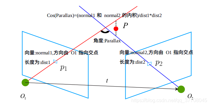
float cosParallax = normal1.dot(normal2)/(dist1*dist2);//三角化的 前方交会角 的余弦值
// Check depth in front of first camera (only if enough parallax, as "infinite" points can easily go to negative depth)
if(p3dC1.at<float>(2)<=0 && cosParallax<0.99998)
continue;
// Check depth in front of second camera (only if enough parallax, as "infinite" points can easily go to negative depth)
cv::Mat p3dC2 = R*p3dC1+t;
//acos(0.99998)=0.3624°,如果 z<0 且 角度变化小于0.3624° , 则舍弃
if(p3dC2.at<float>(2)<=0 && cosParallax<0.99998)
continue;
// Check reprojection error in first image
float im1x, im1y;
float invZ1 = 1.0/p3dC1.at<float>(2);
im1x = fx*p3dC1.at<float>(0)*invZ1+cx;
im1y = fy*p3dC1.at<float>(1)*invZ1+cy;
//计算3d点在第一帧中,投影像素坐标与实际像素坐标的距离平方
float squareError1 = (im1x-kp1.pt.x)*(im1x-kp1.pt.x)+(im1y-kp1.pt.y)*(im1y-kp1.pt.y);
if(squareError1>th2)//如果重投影误差太大,舍弃
continue;
// Check reprojection error in second image
float im2x, im2y;
float invZ2 = 1.0/p3dC2.at<float>(2);
im2x = fx*p3dC2.at<float>(0)*invZ2+cx;
im2y = fy*p3dC2.at<float>(1)*invZ2+cy;
float squareError2 = (im2x-kp2.pt.x)*(im2x-kp2.pt.x)+(im2y-kp2.pt.y)*(im2y-kp2.pt.y);
if(squareError2>th2)
continue;
//至此,3d点成功通过筛选流程,保存 cosParallax 和 p3dC1,统计点的数量
vCosParallax.push_back(cosParallax);
vP3D[vMatches12[i].first] = cv::Point3f(p3dC1.at<float>(0),p3dC1.at<float>(1),p3dC1.at<float>(2));
nGood++;
if(cosParallax<0.99998)
vbGood[vMatches12[i].first]=true;
}
if(nGood>0)//有合格的3d点才进行
{
sort(vCosParallax.begin(),vCosParallax.end());//默认升序
size_t idx = min(50,int(vCosParallax.size()-1));//最大取50
parallax = acos(vCosParallax[idx])*180/CV_PI;//转换为角度,求出所有3d点中的 最小前方交会角 的角度
}
else
parallax=0;
return nGood;
}
其中,计算视差:cosParallax的原理如下图所示:
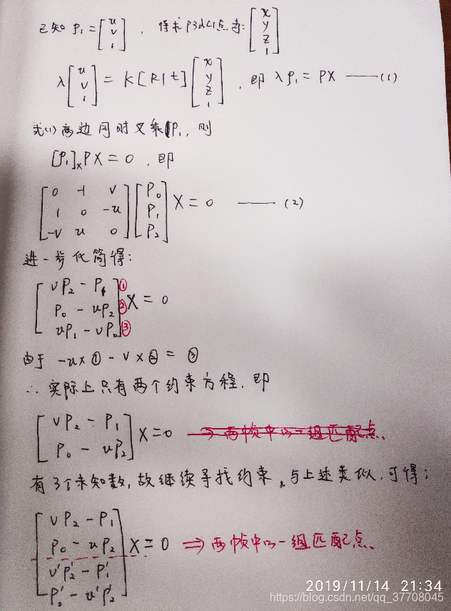
再看看Triangulate(kp1,kp2,P1,P2,p3dC1);函数的原理吧,字有点丑…原谅笔者实在是不想在敲公式了…
(2)基础矩阵恢复
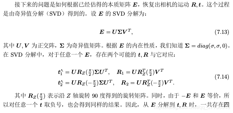
这里我们主要看看如何从基础矩阵F分解出R,t,更准确说是从本质矩阵E,因为源码中将E转换为了F再进行分解的.代码如下:
void Initializer::DecomposeE(const cv::Mat &E, cv::Mat &R1, cv::Mat &R2, cv::Mat &t)
{
    cv::Mat u,w,vt;
    cv::SVD::compute(E,w,u,vt);

    u.col(2).copyTo(t);
    t=t/cv::norm(t);

    cv::Mat W(3,3,CV_32F,cv::Scalar(0));
    W.at<float>(0,1)=-1;
    W.at<float>(1,0)=1;
    W.at<float>(2,2)=1;

    R1 = u*W*vt;
    if(cv::determinant(R1)<0)
        R1=-R1;

    R2 = u*W.t()*vt;
    if(cv::determinant(R2)<0)
        R2=-R2;
}
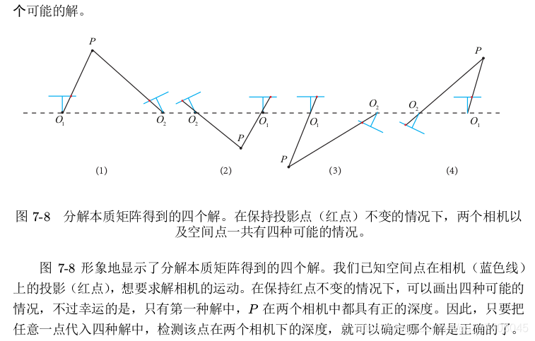
视觉SLAM十四讲是这样讲的…偷个懒…
如若感兴趣关于R,t为何如此取值,可参考博文:https://www.cnblogs.com/FangLai-you/p/10472755.html
关于此处笔者并没有去过多关注.
总结
- 单应矩阵如何分解R,t的理论推导以及源码实现
- 基础矩阵/本质矩阵的理论及其源码实现
参考文献:
- 高翔–视觉SLAM十四讲
- 吴博-ORB-SLAM代码详细解读
PS:
- 如果您觉得我的博客对您有所帮助,欢迎关注我的博客。此外,欢迎转载我的文章,但请注明出处链接。
- 本博客仅代表个人观点,不一定完全正确,如有出错之处,也欢迎批评指正.
上一章节:一步步带你看懂orbslam2源码–单目初始化(三)
下一章节:一步步带你看懂orbslam2源码–单目初始化(五)


 被折叠的 条评论
为什么被折叠?
被折叠的 条评论
为什么被折叠?
 到【灌水乐园】发言


