


Python机器学习基础教程

前言
目前,从医疗诊断和治疗到在社交网络上寻找好友,许多商业应用和研究项目都离不开机
器学习。


第 1 章 引言
本章将解释机器学习如此流行的原因,
并探讨机器学习可以解决哪些类型的问题。
然后将向你展示如何构建第一个机器学习模型,同时介绍一些重要的概念。
1.1 为何选择机器学习

但有了机器学习算法,仅向程序输入海量人脸图像,就足以让算法确定识别人脸需要哪些
特征。
1.1.1 机器学习能够解决的问题
从输入 / 输出对中进行学习的机器学习算法叫作监督学习算法(supervised learning algorithm)
监督机器学习任务的示例:
识别信封上手写的邮政编码
基于医学影像判断肿瘤是否为良性
检测信用卡交易中的诈骗行为
无监督学习算法(unsupervised learning algorithm)
在无监督学习中,只有输入数据是已知的,没有为算法提供输出数据。
无监督学习的示例:
确定一系列博客文章的主题
将客户分成具有相似偏好的群组
检测网站的异常访问模式

1.1.2 熟悉任务和数据

1.2 为何选择 Python

1.3 scikit-learn
1.4 必要的库和工具
1.4.1 Jupyter Notebook
1.4.2 NumPy

1.4.3 SciPy

1.4.4 matplotlib

1.4.5 pandas

1.4.6 mglearn
https://github.com/amueller/introduction_to_ml_with_python

1.5 Python 2 与 Python 3 的对比
1.6 本书用到的版本
1.7 第一个应用:鸢尾花分类

鸢尾花的测量数据:
花瓣的长度
花瓣的宽度
花萼的长度
花萼的宽度
鸢尾花的品种
- setosa
- versicolor
- virginica

单个数据点(一朵鸢尾花)的预期输出是这朵花的品种。对于一个数据点来说,它的品种叫作标签(label)。
1.7.1 初识数据

# 0 加载数据集
from sklearn.datasets import load_iris
iris_dataset = load_iris()

# 1 查看 Iris数据集的keys
print("Iris数据集的keys:",iris_dataset.keys())

# 2 查看数据集的描述信息
print(iris_dataset['DESCR'])
.. _iris_dataset:

Iris plants dataset
--------------------

**Data Set Characteristics:**

    :Number of Instances: 150 (50 in each of three classes)
    :Number of Attributes: 4 numeric, predictive attributes and the class
    :Attribute Information:
        - sepal length in cm
        - sepal width in cm
        - petal length in cm
        - petal width in cm
        - class:
                - Iris-Setosa
                - Iris-Versicolour
                - Iris-Virginica

    :Summary Statistics:

    ============== ==== ==== ======= ===== ====================
                    Min  Max   Mean    SD   Class Correlation
    ============== ==== ==== ======= ===== ====================
    sepal length:   4.3  7.9   5.84   0.83    0.7826
    sepal width:    2.0  4.4   3.05   0.43   -0.4194
    petal length:   1.0  6.9   3.76   1.76    0.9490  (high!)
    petal width:    0.1  2.5   1.20   0.76    0.9565  (high!)
    ============== ==== ==== ======= ===== ====================

    :Missing Attribute Values: None
    :Class Distribution: 33.3% for each of 3 classes.
    :Creator: R.A. Fisher
    :Donor: Michael Marshall (MARSHALL%PLU@io.arc.nasa.gov)
    :Date: July, 1988

The famous Iris database, first used by Sir R.A. Fisher. The dataset is taken
from Fisher's paper. Note that it's the same as in R, but not as in the UCI
Machine Learning Repository, which has two wrong data points.

This is perhaps the best known database to be found in the
pattern recognition literature.  Fisher's paper is a classic in the field and
is referenced frequently to this day.  (See Duda & Hart, for example.)  The
data set contains 3 classes of 50 instances each, where each class refers to a
type of iris plant.  One class is linearly separable from the other 2; the
latter are NOT linearly separable from each other.

.. topic:: References

   - Fisher, R.A. "The use of multiple measurements in taxonomic problems"
     Annual Eugenics, 7, Part II, 179-188 (1936); also in "Contributions to
     Mathematical Statistics" (John Wiley, NY, 1950).
   - Duda, R.O., & Hart, P.E. (1973) Pattern Classification and Scene Analysis.
     (Q327.D83) John Wiley & Sons.  ISBN 0-471-22361-1.  See page 218.
   - Dasarathy, B.V. (1980) "Nosing Around the Neighborhood: A New System
     Structure and Classification Rule for Recognition in Partially Exposed
     Environments".  IEEE Transactions on Pattern Analysis and Machine
     Intelligence, Vol. PAMI-2, No. 1, 67-71.
   - Gates, G.W. (1972) "The Reduced Nearest Neighbor Rule".  IEEE Transactions
     on Information Theory, May 1972, 431-433.
   - See also: 1988 MLC Proceedings, 54-64.  Cheeseman et al"s AUTOCLASS II
     conceptual clustering system finds 3 classes in the data.
   - Many, many more ...


监督学习
1.7.2 衡量模型是否成功:训练数据与测试数据

from sklearn.model_selection import train_test_split
X_train,X_test,y_train,y_test = train_test_split(iris_dataset['data'],iris_dataset['target'],random_state=0)
print("训练集X_train.shape = ",X_train.shape)
print("训练集y_train.shape = ",y_train.shape)
print("测试集X_test.shape = ",X_test.shape)
print("测试集y_test.shape = ",y_test.shape)

1.7.3 要事第一:观察数据

1.7.4 构建第一个模型:k 近邻算法

1.7.5 做出预测
import numpy as np
X_new = np.array([[5,2.9,1,0.2]])
prediction = knn.predict(X_new)
print(prediction)
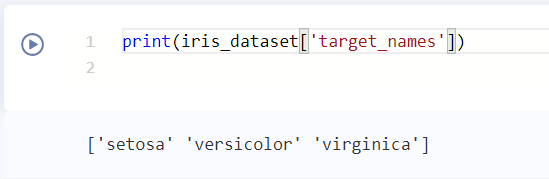
print(iris_dataset['target_names'][prediction])

1.7.6 评估模型
y_pred = knn.predict(X_test)
print(np.mean(y_pred == y_test))  #求取均值

1.8 小结与展望

第 2 章 监督学习
2.1 分类与回归 .21
2.2 泛化、过拟合与欠拟合 .22
2.3 监督学习算法 .24
2.3.1 一些样本数据集 25
2.3.2 k 近邻 .28
2.3.3 线性模型 35
2.3.4 朴素贝叶斯分类器 53
2.3.5 决策树 54
2.3.6 决策树集成 64
2.3.7 核支持向量机 71
2.3.8 神经网络(深度学习) 80
2.4 分类器的不确定度估计 .91
2.4.1 决策函数 91
2.4.2 预测概率 94
2.4.3 多分类问题的不确定度 96
2.5 小结与展望 .98
第 3 章 无监督学习与预处理100
3.1 无监督学习的类型 .100
3.2 无监督学习的挑战 .101
3.3 预处理与缩放 .101
3.3.1 不同类型的预处理 102
3.3.2 应用数据变换 102
3.3.3 对训练数据和测试数据进行相同的缩放 104
3.3.4 预处理对监督学习的作用 106
3.4 降维、特征提取与流形学习 .107
3.4.1 主成分分析 107
3.4.2 非负矩阵分解 120
3.4.3 用 t-SNE 进行流形学习 126
3.5 聚类 .130
3.5.1 k 均值聚类 .130
3.5.2 凝聚聚类 140
3.5.3 DBSCAN 143
3.5.4 聚类算法的对比与评估 147
3.5.5 聚类方法小结 159
3.6 小结与展望 .159
第 4 章 数据表示与特征工程161
4.1 分类变量 .161
4.1.1 One-Hot 编码(虚拟变量) .162
4.1.2 数字可以编码分类变量 166
4.2 分箱、离散化、线性模型与树 .168
4.3 交互特征与多项式特征 .171
4.4 单变量非线性变换 .178
4.5 自动化特征选择 .181
4.5.1 单变量统计 181
4.5.2 基于模型的特征选择 183
4.5.3 迭代特征选择 184
4.6 利用专家知识 .185
4.7 小结与展望 .192
第 5 章 模型评估与改进 193
5.1 交叉验证 .194
5.1.1 scikit-learn 中的交叉验证 194
5.1.2 交叉验证的优点 195
5.1.3 分层 k 折交叉验证和其他策略 .196
5.2 网格搜索 .200
5.2.1 简单网格搜索 201
5.2.2 参数过拟合的风险与验证集 202
5.2.3 带交叉验证的网格搜索 203
5.3 评估指标与评分 .213
5.3.1 牢记最终目标 213
5.3.2 二分类指标 214
5.3.3 多分类指标 230
5.3.4 回归指标 232
5.3.5 在模型选择中使用评估指标 232
5.4 小结与展望 .234
第 6 章 算法链与管道 .236
6.1 用预处理进行参数选择 .237
6.2 构建管道 .238
6.3 在网格搜索中使用管道 .239
6.4 通用的管道接口 .242
6.4.1 用 make_pipeline 方便地创建管道 .243
6.4.2 访问步骤属性 244
6.4.3 访问网格搜索管道中的属性 244
6.5 网格搜索预处理步骤与模型参数 .246
6.6 网格搜索选择使用哪个模型 .248
6.7 小结与展望 .249
第 7 章 处理文本数据 .250
7.1 用字符串表示的数据类型 .250
7.2 示例应用:电影评论的情感分析 .252
7.3 将文本数据表示为词袋 .254
7.3.1 将词袋应用于玩具数据集 255
7.3.2 将词袋应用于电影评论 256
7.4 停用词 .259
7.5 用 tf-idf 缩放数据 260
7.6 研究模型系数 .263
7.7 多个单词的词袋(n 元分词) 263
7.8 高级分词、词干提取与词形还原 .267
7.9 主题建模与文档聚类 .270
7.10 小结与展望 .277
第 8 章 全书总结 278
8.1 处理机器学习问题 .278
8.2 从原型到生产 .279
8.3 测试生产系统 .280
8.4 构建你自己的估计器 .280
8.5 下一步怎么走 .281
8.5.1 理论 281
8.5.2 其他机器学习框架和包 281
8.5.3 排序、推荐系统与其他学习类型 282
8.5.4 概率建模、推断与概率编程 282
8.5.5 神经网络 283
8.5.6 推广到更大的数据集 283
8.5.7 磨练你的技术 284
8.6 总结 .284


 2172
2172


 被折叠的 条评论
为什么被折叠?
被折叠的 条评论
为什么被折叠?
 到【灌水乐园】发言


