扩散模型（三）：基于UNet2DModel的扩散模型算法搭建

前言：学习了扩散模型从原理到实战-异步社区-致力于优质IT知识的出版和分享 (epubit.com)这本教材后，对教材里所提的内容进行了自我消化，总结总结。

UNet2DModel比BasicUNet模型根伟先进，相比于BasicUnet做了如下改进：

• GroupNorm层对每个模块的输入进行组标准化
• Dropout层使的训练更加平滑
• 每个块具有多个ResNet层
• 引入了注意力机制
• 可以对时间步进行调节
• 具有可学习参数的上采样模块和下采样模块

创建一个UNet2DModel模块：

import torch
import torchvision
from torch import nn
from torch.nn import functional as F
from torch.utils.data import DataLoader
from diffusers import DDPMScheduler, UNet2DModel
from matplotlib import pyplot as plt

net = UNet2DModel(
    sample_size=28,  # the target image resolution
    in_channels=1,  # the number of input channels, 3 for RGB images
    out_channels=1,  # the number of output channels
    layers_per_block=2,  # how many ResNet layers to use per UNet block
    block_out_channels=(32, 64, 64),  # Roughly matching our basic unet example
    down_block_types=(
        "DownBlock2D",  # a regular ResNet downsampling block
        "AttnDownBlock2D",  # a ResNet downsampling block with spatial self-attention
        "AttnDownBlock2D",
    ),
    up_block_types=(
        "AttnUpBlock2D",
        "AttnUpBlock2D",  # a ResNet upsampling block with spatial self-attention
        "UpBlock2D",   # a regular ResNet upsampling block
      ),
)

print(net)

很明显，UNet2DModel模块相比于BasicUNet更为复杂，使用了约170万个参数（BasicUNet使用了30多万个）。只需要在扩散模型基础（一）：基于BasicUNet的扩散模型算法搭建-CSDN博客 算法的基础上，将BasicUNet更换为UNet2DModel，并修改采样预测的过程即可。

调试好的全套算法如下：

import torch
import torchvision
from torch import nn
from torch.nn import functional as F
from torch.utils.data import DataLoader
from diffusers import DDPMScheduler, UNet2DModel
from matplotlib import pyplot as plt

device = torch.device("cuda" if torch.cuda.is_available() else "cpu")
print(f'Using device: {device}')

dataset = torchvision.datasets.MNIST(root="mnist/", train=True, download=True, transform=torchvision.transforms.ToTensor())

train_dataloader = DataLoader(dataset, batch_size=8, shuffle=True)

# Dataloader (you can mess with batch size)
batch_size = 128
train_dataloader = DataLoader(dataset, batch_size=batch_size, shuffle=True)

# How many runs through the data should we do?
n_epochs = 3

def corrupt(x, amount):
  """Corrupt the input `x` by mixing it with noise according to `amount`"""

  #print(amount)

  noise = torch.rand_like(x)

  #print(noise)

  amount = amount.view(-1, 1, 1, 1) # Sort shape so broadcasting works

  #print(amount)

  return x*(1-amount) + noise*amount

# Create the network
net = UNet2DModel(
    sample_size=28,  # the target image resolution
    in_channels=1,  # the number of input channels, 3 for RGB images
    out_channels=1,  # the number of output channels
    layers_per_block=2,  # how many ResNet layers to use per UNet block
    block_out_channels=(32, 64, 64),  # Roughly matching our basic unet example
    down_block_types=(
        "DownBlock2D",  # a regular ResNet downsampling block
        "AttnDownBlock2D",  # a ResNet downsampling block with spatial self-attention
        "AttnDownBlock2D",
    ),
    up_block_types=(
        "AttnUpBlock2D",
        "AttnUpBlock2D",  # a ResNet upsampling block with spatial self-attention
        "UpBlock2D",   # a regular ResNet upsampling block
      ),
) #<<<
net.to(device)

# Our loss finction
loss_fn = nn.MSELoss()

# The optimizer
opt = torch.optim.Adam(net.parameters(), lr=1e-3)

# Keeping a record of the losses for later viewing
losses = []

# The training loop
for epoch in range(n_epochs):

    for x, y in train_dataloader:

        # Get some data and prepare the corrupted version
        x = x.to(device) # Data on the GPU
        noise_amount = torch.rand(x.shape[0]).to(device) # Pick random noise amounts
        noisy_x = corrupt(x, noise_amount) # Create our noisy x

        # Get the model prediction
        pred = net(noisy_x, 0).sample #<<< Using timestep 0 always, adding .sample

        # Calculate the loss
        loss = loss_fn(pred, x) # How close is the output to the true 'clean' x?

        # Backprop and update the params:
        opt.zero_grad()
        loss.backward()
        opt.step()

        # Store the loss for later
        losses.append(loss.item())

    # Print our the average of the loss values for this epoch:
    avg_loss = sum(losses[-len(train_dataloader):])/len(train_dataloader)
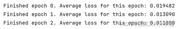
    print(f'Finished epoch {epoch}. Average loss for this epoch: {avg_loss:05f}')

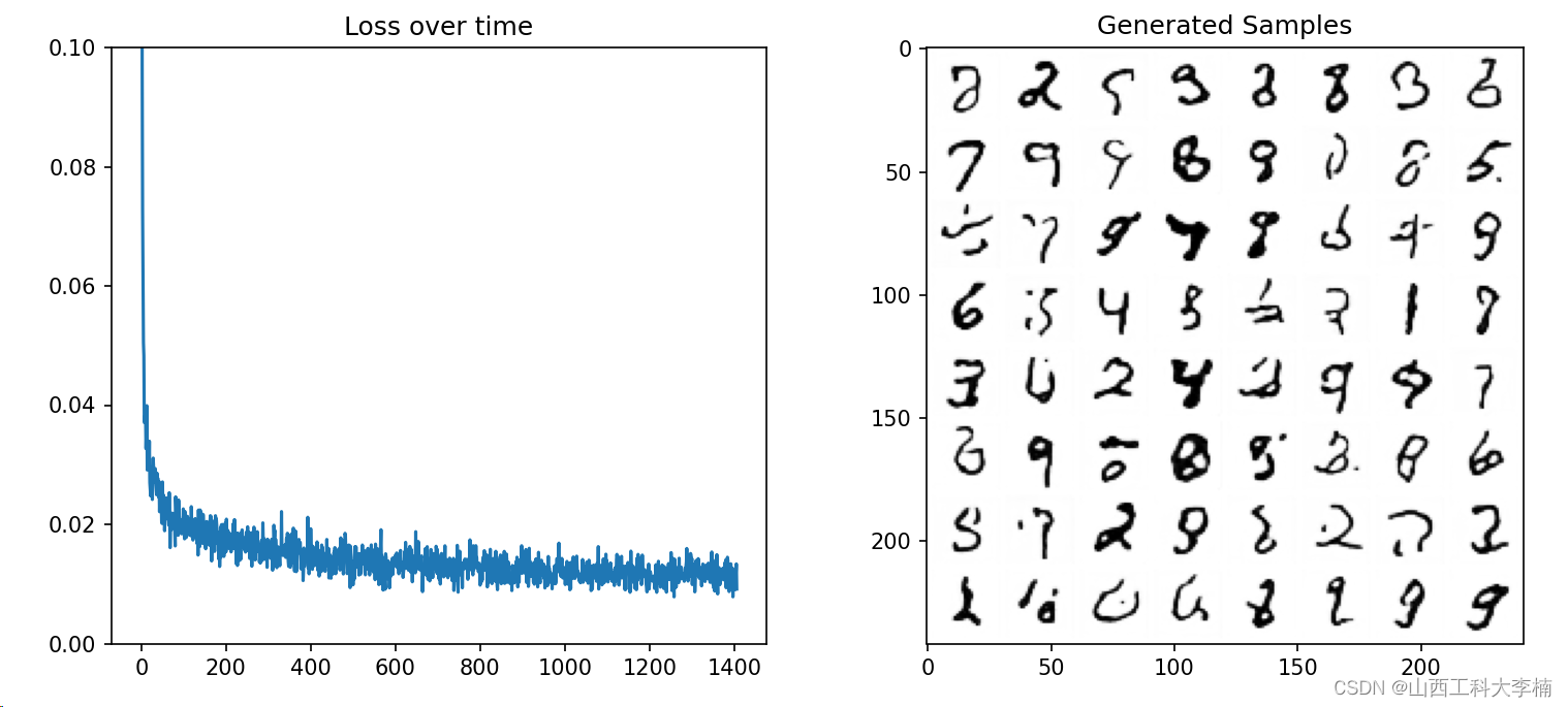
# Plot losses and some samples
fig, axs = plt.subplots(1, 2, figsize=(12, 5))

# Losses
axs[0].plot(losses)
axs[0].set_ylim(0, 0.1)
axs[0].set_title('Loss over time')

# Samples
n_steps = 40
x = torch.rand(64, 1, 28, 28).to(device)
for i in range(n_steps):
  noise_amount = torch.ones((x.shape[0], )).to(device) * (1-(i/n_steps)) # Starting high going low
  with torch.no_grad():
    pred = net(x, 0).sample
  mix_factor = 1/(n_steps - i)
  x = x*(1-mix_factor) + pred*mix_factor

axs[1].imshow(torchvision.utils.make_grid(x.detach().cpu(), nrow=8)[0].clip(0, 1), cmap='Greys')
axs[1].set_title('Generated Samples');

plt.show()

运行结果：