


Backtrader 文档学习-Data Feeds
1.数据载入
Quickstart中已经学习了基础的数据载入到cerebro中。
- self.datas 是按插入顺序的数组
- 数组对象的别名
- self.data 和 self.data0 一样,都是指向第一组数据
- self.dataX 指向第N组数据
import backtrader as bt
import backtrader.feeds as btfeeds

data = btfeeds.YahooFinanceCSVData(dataname='wheremydatacsvis.csv')

cerebro = bt.Cerebro()

cerebro.adddata(data)  # a 'name' parameter can be passed for plotting purposes
从github上下载BackTrader包,有用例中提供的所有的测试数据,有txt和csv的数据版本:
# ll
total 3436
-rw-r--r--. 1 root root   24109 Apr 19  2023 2005-2006-day-001.txt
-rw-r--r--. 1 root root 1820067 Apr 19  2023 2006-01-02-volume-min-001.txt
-rw-r--r--. 1 root root   15123 Apr 19  2023 2006-day-001-optix.txt
-rw-r--r--. 1 root root   12030 Apr 19  2023 2006-day-001.txt
-rw-r--r--. 1 root root    6108 Apr 19  2023 2006-day-002.txt
-rw-r--r--. 1 root root  120002 Apr 19  2023 2006-min-005.txt
-rw-r--r--. 1 root root     609 Apr 19  2023 2006-month-001.txt
-rw-r--r--. 1 root root   15130 Apr 19  2023 2006-volume-day-001.txt
-rw-r--r--. 1 root root    2489 Apr 19  2023 2006-week-001.txt
-rw-r--r--. 1 root root    1267 Apr 19  2023 2006-week-002.txt
-rw-r--r--. 1 root root     543 Apr 19  2023 bidask2.csv
-rw-r--r--. 1 root root     358 Apr 19  2023 bidask.csv
-rw-r--r--. 1 root root  272573 Apr 19  2023 nvda-1999-2014.txt
-rw-r--r--. 1 root root   17462 Apr 19  2023 nvda-2014.txt
-rw-r--r--. 1 root root  345989 Apr 19  2023 orcl-1995-2014.txt
-rw-r--r--. 1 root root   52877 Apr 19  2023 orcl-2003-2005.txt
-rw-r--r--. 1 root root   17638 Apr 19  2023 orcl-2014.txt
-rw-r--r--. 1 root root    8207 Apr 19  2023 ticksample.csv
-rw-r--r--. 1 root root  324337 Apr 19  2023 yhoo-1996-2014.txt
-rw-r--r--. 1 root root  341934 Apr 19  2023 yhoo-1996-2015.txt
-rw-r--r--. 1 root root   52718 Apr 19  2023 yhoo-2003-2005.txt
-rw-r--r--. 1 root root   17666 Apr 19  2023 yhoo-2014.txt
2. 数据载入的常用参数
参数:
- dataname (默认: None) - 必须提供。含义随数据馈送类型(文件位置,代码等)而异。
- name (默认: ‘’) - 绘图中用于装饰目的的意思。如果未指定,则可以从数据名派生(例如:文件路径的最后一部分)。
- fromdate (默认: mindate) - Python datetime对象,指示应忽略此日期之前的任何datetime。
- todate (默认: maxdate) - Python datetime对象,指示该日期之后的任何datetime应该被忽略。
- timeframe (默认是TimeFrame.Days), 其他可以设置的值: Ticks, Seconds, Minutes, Days, Weeks, Months and Years
- compression (默认是1),从实际的bar中取有效的bar,提供有用信息的仅在数据重新采样/回放中有效。
- sessionstart (默认None),指示数据的会话开始时间。可以由类用于重新采样等目的。
- sessionend (默认None),指示数据的会话结束时间。可以由类用于重新采样等目的。
3.CSV分隔符
- headers (默认True)指示传递的数据是否具有初始标题行
- separator (默认分隔符,)用于标记每个CSV行分割
3. GenericCSVData方法
参数说明:
- dataname (默认: None) - CSV 文件的路径或文件名。这是必需的参数,用于指定要加载的 CSV 文件的位置。
- datetime (默认: 0) - CSV 文件中包含日期时间的列的索引。 BackTrader 哪一列包含日期时间信息。
- open (默认: 1) - CSV 文件中包含开盘价的列的索引。 BackTrader 哪一列包含开盘价数据。
- high (默认: 2) - CSV 文件中包含最高价的列的索引。 BackTrader 哪一列包含最高价数据。
- low (默认: 3) - CSV 文件中包含最低价的列的索引。 BackTrader 哪一列包含最低价数据。
- close (默认: 4) - CSV 文件中包含收盘价的列的索引。 BackTrader 哪一列包含收盘价数据。
- volume (默认: 5) - CSV 文件中包含成交量的列的索引。可选参数,用于指定成交量数据所在的列。
- openinterest (默认: 6) - CSV 文件中包含持仓量的列的索引。可选参数,用于指定持仓量数据所在的列。
- nullvalue (默认: float(‘NaN’))如果缺少应存在的值(CSV字段为空),将指定使用值替代。
- dtformat (默认: ‘%Y-%m-%d’) - 日期时间格式字符串。用于解析 CSV 文件中的日期时间数据。
- nullvalue (默认: float(‘NaN’))如果缺少应存在的值(CSV字段为空),将指定使用值替代。
- dtformat (默认: ‘%Y-%m-%d’) 日期时间格式字符串。用于解析 CSV 文件中的日期数据。
- tmformat (默认: %H:%M:%S) 时间格式字符串。用于解析 CSV 文件中的时间数据。
import datetime
import backtrader as bt
import backtrader.feeds as btfeeds

...
...

data = btfeeds.GenericCSVData(
    dataname='mydata.csv',

    fromdate=datetime.datetime(2000, 1, 1),
    todate=datetime.datetime(2000, 12, 31),

    nullvalue=0.0,

    dtformat=('%Y-%m-%d'),

    datetime=0,
    high=1,
    low=2,
    open=3,
    close=4,
    volume=5,
    openinterest=-1
)

...
说明:
- 限制输入到2000年
- 顺序是HLOC而不是OHLC
- 缺失值用0替代
- 日线的日期格式是YYYY-MM-DD
- 当前数据没有openinterest 值
也可以子类参数定义导入csv文件
import datetime
import backtrader.feeds as btfeed

class MyHLOC(btfreeds.GenericCSVData):

  params = (
    ('fromdate', datetime.datetime(2000, 1, 1)),
    ('todate', datetime.datetime(2000, 12, 31)),
    ('nullvalue', 0.0),
    ('dtformat', ('%Y-%m-%d')),
    ('tmformat', ('%H.%M.%S')),

    ('datetime', 0),
    ('time', 1),
    ('high', 2),
    ('low', 3),
    ('open', 4),
    ('close', 5),
    ('volume', 6),
    ('openinterest', -1)
)
4.扩展数据导入
除了OHLC之外,能否提供自定义的列 ,当然可以。
增加PE列:
from backtrader.feeds import GenericCSVData

class GenericCSV_PE(GenericCSVData):

    # Add a 'pe' line to the inherited ones from the base class
    lines = ('pe',)

    # openinterest in GenericCSVData has index 7 ... add 1
    # add the parameter to the parameters inherited from the base class
    params = (('pe', 8),)
使用PE数据
import backtrader as bt

....

class MyStrategy(bt.Strategy):

    ...

    def next(self):

        if self.data.close > 2000 and self.data.pe < 12:
            # TORA TORA TORA --- Get off this market
            self.sell(stake=1000000, price=0.01, exectype=Order.Limit)
    ...
用PE数据做图
import backtrader as bt
import backtrader.indicators as btind

....

class MyStrategy(bt.Strategy):

    def __init__(self):

        # The indicator autoregisters and will plot even if no obvious
        # reference is kept to it in the class
        btind.SMA(self.data.pe, period=1, subplot=False)

    ...

    def next(self):

        if self.data.close > 2000 and self.data.pe < 12:
            # TORA TORA TORA --- Get off this market
            self.sell(stake=1000000, price=0.01, exectype=Order.Limit)
    ...
5. CSV导入
CSV Data Feed Development 和 Binary Datafeed Development
两节都是深入的CSV数据导入的细节,暂时不用,实际还是从库里加载数据比较方便。。
6.多周期导入
投资决策需要使用不同的时间区间
- 周线用于评估趋势
- 日线用于执行投资
或者是5分钟线和60分钟线
BackTrader原生支持不同的时间区间,用户需遵循以下规则: - 最小的时间区间数据(也就是数据量最多的)应第一个被加载到cerebro中
- 数据的日期必须对齐一致,平台才能理解处理
用户可以随意应用indicator处理更短或更长的时间区间。
- 指示器应用长的时间区间产生更少的数据bar
- 最小时间区间的数据可以用于更长的时间区间
看最后的总结示例(程序命名multitimeframe-example.py),统一演示。
需要注意原始示例中:
parser.add_argument(‘–timeframe’, default=‘weekly’, required=False,
choices=[‘daily’, ‘weekly’, ‘monhtly’],
monhtly拼写错误,月线执行会报错,修改monthly。
from __future__ import (absolute_import, division, print_function,
                        unicode_literals)

import argparse

import backtrader as bt
import backtrader.feeds as btfeeds
import backtrader.indicators as btind


class SMAStrategy(bt.Strategy):
    params = (
        ('period', 10),
        ('onlydaily', False),
    )

    def __init__(self):
        self.sma_small_tf = btind.SMA(self.data, period=self.p.period)
        if not self.p.onlydaily:
            self.sma_large_tf = btind.SMA(self.data1, period=self.p.period)

    def nextstart(self):
        print('--------------------------------------------------')
        print('nextstart called with len', len(self))
        print('--------------------------------------------------')

        super(SMAStrategy, self).nextstart()


def runstrat():
    args = parse_args()

    # Create a cerebro entity
    cerebro = bt.Cerebro(stdstats=False)

    # Add a strategy
    if not args.indicators:
        cerebro.addstrategy(bt.Strategy)
    else:
        cerebro.addstrategy(
            SMAStrategy,

            # args for the strategy
            period=args.period,
            onlydaily=args.onlydaily,
        )

    # Load the Data
    datapath = args.dataname or '../../datas/2006-day-001.txt'
    data = btfeeds.BacktraderCSVData(dataname=datapath)
    cerebro.adddata(data)  # First add the original data - smaller timeframe

    tframes = dict(daily=bt.TimeFrame.Days, weekly=bt.TimeFrame.Weeks,
                   monthly=bt.TimeFrame.Months)

    # Handy dictionary for the argument timeframe conversion
    # Resample the data
    if args.noresample:
        datapath = args.dataname2 or '../../datas/2006-week-001.txt'
        data2 = btfeeds.BacktraderCSVData(dataname=datapath)
        # And then the large timeframe
        cerebro.adddata(data2)
    else:
        cerebro.resampledata(data, timeframe=tframes[args.timeframe],
                             compression=args.compression)

    # Run over everything
    cerebro.run()

    # Plot the result
    cerebro.plot(style='bar')


def parse_args():
    parser = argparse.ArgumentParser(
        description='Multitimeframe test')

    parser.add_argument('--dataname', default='', required=False,
                        help='File Data to Load')

    parser.add_argument('--dataname2', default='', required=False,
                        help='Larger timeframe file to load')

    parser.add_argument('--noresample', action='store_true',
                        help='Do not resample, rather load larger timeframe')

    parser.add_argument('--timeframe', default='weekly', required=False,
                        choices=['daily', 'weekly', 'monthly'],
                        help='Timeframe to resample to')

    parser.add_argument('--compression', default=1, required=False, type=int,
                        help='Compress n bars into 1')

    parser.add_argument('--indicators', action='store_true',
                        help='Wether to apply Strategy with indicators')

    parser.add_argument('--onlydaily', action='store_true',
                        help='Indicator only to be applied to daily timeframe')

    parser.add_argument('--period', default=10, required=False, type=int,
                        help='Period to apply to indicator')

    return parser.parse_args()


if __name__ == '__main__':
    runstrat()
调用参数的设置很好,值得学习。
说明:
- 使用git下载的示例数据,把程序放在和datas目录外
- 核心是下面一段程序
如果没有参数,复制数据加载到cerebro中,cerebro中有两个一样的数据
如果有参数,参数带入到resampledata方法中执行
最后做图
    if args.noresample:
        datapath = args.dataname2 or '../../datas/2006-week-001.txt'
        data2 = btfeeds.BacktraderCSVData(dataname=datapath)
        # And then the large timeframe
        cerebro.adddata(data2)
    else:
        cerebro.resampledata(data, timeframe=tframes[args.timeframe],
                             compression=args.compression)
- 通过变化参数,理解resampledata方法:
(1)参数help
python ./multitimeframe-example.py --help
usage: multitimeframe-example.py [-h] [--dataname DATANAME]
                                 [--dataname2 DATANAME2] [--noresample]
                                 [--timeframe {daily,weekly,monthly}]
                                 [--compression COMPRESSION] [--indicators]
                                 [--onlydaily] [--period PERIOD]

Multitimeframe test

optional arguments:
  -h, --help            show this help message and exit
  --dataname DATANAME   File Data to Load
  --dataname2 DATANAME2
                        Larger timeframe file to load
  --noresample          Do not resample, rather load larger timeframe
  --timeframe {daily,weekly,monthly}
                        Timeframe to resample to
  --compression COMPRESSION
                        Compress n bars into 1
  --indicators          Wether to apply Strategy with indicators
  --onlydaily           Indicator only to be applied to daily timeframe
  --period PERIOD       Period to apply to indicator
(2)周线
python ./multitimeframe-example.py --timeframe weekly --compression 1

周线
(3)日线压缩
python ./multitimeframe-example.py --timeframe daily --compression 2
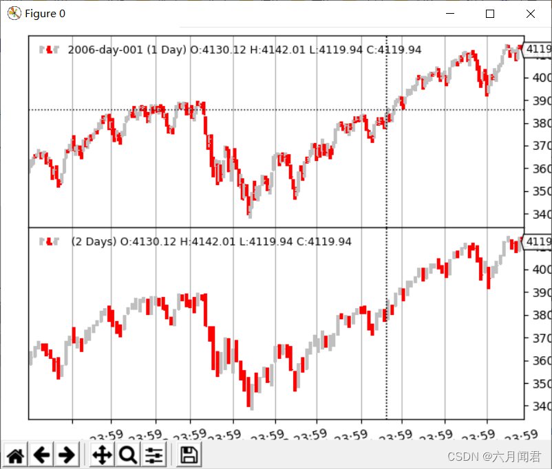
日线压缩2倍
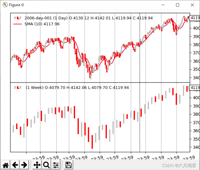
(4)使用日线SMA
python ./multitimeframe-example.py --timeframe weekly --compression 1 --indicators --onlydaily
--------------------------------------------------
nextstart called with len 10
--------------------------------------------------
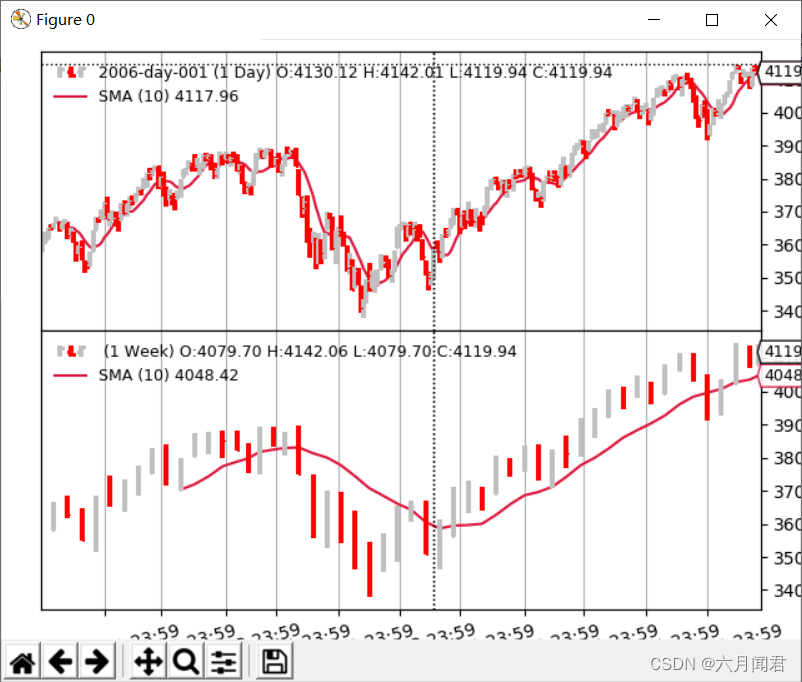
(5)指示器压缩周线
- 策略不是在10个周期后调用,而是在50个周期后第一次调用。 是因为在更长的(每周)时间框架上应用的简单移动平均线在10周后产生一个值,即10周* 5天/周=50天,nextstart第一个长度是51 。
- nextstart执行5次
是混合时间区间的自然副作用,在这种情况下,指标只应用于更大的时间区间。 较大的时间框架简单移动平均线产生5倍的相同价值,同时消耗5根日线。 SMA的默认周期是10,指示器受控于更大的时间区间。
python ./multitimeframe-example.py --timeframe weekly --compression 1 --indicators
--------------------------------------------------
nextstart called with len 51
--------------------------------------------------
--------------------------------------------------
nextstart called with len 52
--------------------------------------------------
--------------------------------------------------
nextstart called with len 53
--------------------------------------------------
--------------------------------------------------
nextstart called with len 54
--------------------------------------------------
--------------------------------------------------
nextstart called with len 55
--------------------------------------------------
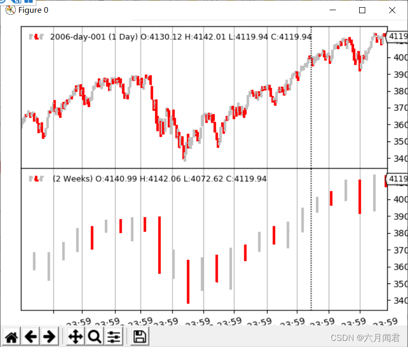
(6)周线压缩
python ./multitimeframe-example.py --timeframe weekly --compression 2
(7)月线
python ./multitimeframe-example.py --timeframe monthly --compression 1


 572
572


 被折叠的 条评论
为什么被折叠?
被折叠的 条评论
为什么被折叠?
 到【灌水乐园】发言


