


《机器学习实战》斧头书——决策树
一、对文章的说明
1.1 对本文有几点说明如下:
1.1.1 我是一个刚学没多久的小白,所以代码可能也会有错误,欢迎各位大佬提出我的问题,感谢;
1.1.2 对于python版本 ,斧头书《机器学习实战》是用的2.x,本文使用的是3.x,然后代码的话,有的是参考书上的和网上的,还有部分是自己写的;
1.1.3 用的参考书是下面这本,封面拿了个斧头的人,这本书没有调库,都是用python写的底层代码,感觉对理解算法原理会更深入一点;
1.1.4 编写代码的地方,先是在Jupyter notebook上编写和部分代码的测试,最后在PyCharm上集成和封装。

二、项目背景
2.1 背景1
本节我们将通过一个例子讲解决策树如何预测患者需要佩戴的隐形眼镜类型。使用小数据集,我们就可以利用决策树学到很多知识:眼科医生是如何判断患者需要佩戴的镜片类型;一旦理解了决策树的工作原理,我们甚至也可以帮助人们判断需要佩戴的镜片类型。
2.2 背景2
隐形眼镜数据集是非常著名的数据集,它包含很多患者眼部状况的观察条件以及医生推荐的隐形眼镜类型。隐形眼镜类型包括硬材质、软材质以及不适合佩戴隐形眼镜。
2.3 熵的计算公式
先是信息的定义:
再是熵,熵就是信息的期望值(期望值就是平均值):

三、代码
3.1 隐形眼镜的数据集
astigmatic是散光的意思;myope是近视眼,hyper是更加近视,最后labels是根据前面的条件判断你是“不需要带隐形眼镜”还是“带软的”还是“带硬的”。
    age	 	 prescript	astigmatic	tearRate	labels
0	young		myope	no			reduced		no lenses
1	young		myope	no			normal		soft
2	young		myope	yes			reduced		no lenses
3	young		myope	yes			normal		hard
4	young		hyper	no			reduced		no lenses
5	young		hyper	no			normal		soft
6	young		hyper	yes			reduced		no lenses
7	young		hyper	yes			normal		hard
8	pre			myope	no			reduced		no lenses
9	pre			myope	no			normal		soft
10	pre			myope	yes			reduced		no lenses
11	pre			myope	yes			normal		hard
12	pre			hyper	no			reduced		no lenses
13	pre			hyper	no			normal		soft
14	pre			hyper	yes			reduced		no lenses
15	pre			hyper	yes			normal		no lenses
16	presbyopic	myope	no			reduced		no lenses
17	presbyopic	myope	no			normal		no lenses
18	presbyopic	myope	yes			reduced		no lenses
19	presbyopic	myope	yes			normal		hard
20	presbyopic	hyper	no			reduced		no lenses
21	presbyopic	hyper	no			normal		soft
22	presbyopic	hyper	yes			reduced		no lenses
23	presbyopic	hyper	yes			normal		no lenses
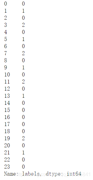
#将标称型数据  转换成  数值型,否则无法用sklearn库画图。
age	prescript	astigmatic	tearRate
0	0	0	0	0
1	0	0	0	1
2	0	0	1	0
3	0	0	1	1
4	0	1	0	0
5	0	1	0	1
6	0	1	1	0
7	0	1	1	1
8	1	0	0	0
9	1	0	0	1
10	1	0	1	0
11	1	0	1	1
12	1	1	0	0
13	1	1	0	1
14	1	1	1	0
15	1	1	1	1
16	2	0	0	0
17	2	0	0	1
18	2	0	1	0
19	2	0	1	1
20	2	1	0	0
21	2	1	0	1
22	2	1	1	0
23	2	1	1	1
这是数值型的labels
3.2 先是计算熵增部分的代码(根据公式编程)
import numpy as np
import pandas as pd
import matplotlib.pyplot as plt
#创建数据集
dataSet = pd.read_csv('lenses.txt',sep='\t',names=['age','prescript','astigmatic','tearRate','labels'])
#从当前文件夹读取数据
#这里数据的分隔符sep是Tab,即\t。添加列名names
def calEnt(dataSet): #计算信息熵的函数
    n = dataSet.shape[0] #数据集总行数
    iset = dataSet.iloc[:,-1].value_counts() #标签的所有类别
    p = iset/n #每一类标签所占比
    ent = (-p*np.log2(p)).sum() #计算信息熵
    return ent
def bestSplit(dataSet):#选择最优的列进行切分的函数
    baseEnt = calEnt(dataSet) #计算原始熵
    bestGain = 0 #初始化信息增益
    axis = -1 #初始化最佳切分列,标签列
    for i in range(dataSet.shape[1]-1): #对特征的每一列进行循环   1和0
        levels= dataSet.iloc[:,i].value_counts().index #提取出当前列的所有取值
        ents = 0 #初始化子节点的信息熵
        for j in levels: #对当前列的每一个取值进行循环    j=1和0
            childSet = dataSet[dataSet.iloc[:,i]==j] #某一个子节点的dataframe
            # print("childSet:\n",childSet)
            ent = calEnt(childSet) #计算某一个子节点的信息熵
            ents += (childSet.shape[0]/dataSet.shape[0])*ent #计算当前列的信息熵
            # print(f'第{i}列的信息熵为{ents}')
        infoGain = baseEnt-ents #计算当前列的信息增益
        # print(f'第{i}列的信息增益为{infoGain}')
        if (infoGain > bestGain):
            bestGain = infoGain #选择最大信息增益
            axis = i #最大信息增益所在列的索引
    return axis
def mySplit(dataSet,axis,value): #选择某一列和某一值进行分割
    col = dataSet.columns[axis]
    rest_dataSet = dataSet.loc[dataSet[col]==value,:].drop(col,axis=1)
    return rest_dataSet
def createTree(dataSet): #创建决策树的函数
    featlist = list(dataSet.columns) #提取出数据集所有的列
    classlist = dataSet.iloc[:,-1].value_counts() #获取最后一列类标签
    #最多标签数目是否等于数据集行数,或者数据集是否只有一列的时候就直接返回
    if classlist[0]==dataSet.shape[0] or dataSet.shape[1] == 1:
        return classlist.index[0] #如果是,返回类标签
    axis = bestSplit(dataSet) #确定出当前最佳切分列的索引
    bestfeat = featlist[axis] #获取该索引对应的特征
    myTree = {bestfeat:{}} #采用字典嵌套的方式存储树信息
    del featlist[axis] #删除当前特征,因为用完了下次就不会再用了
    valuelist = set(dataSet.iloc[:,axis]) #提取最佳切分列所有属性值
    for value in valuelist: #对每一个属性值递归建树
        myTree[bestfeat][value] = createTree(mySplit(dataSet,axis,value))
    return myTree
myTree_lenses = createTree(dataSet)
#把决策树存储起来
np.save('myTree_lenses.npy',myTree_lenses)
#决策树的读取  不加.item()的话,输出的是array格式,加了就提取里面的内容了。allow_pickle=True要加,不然会报错。
read_myTree_lenses = np.load('myTree_lenses.npy',allow_pickle=True).item()
def classify(inputTree,labels,testVec):
    firstStr = next(iter(inputTree)) #获取决策树第一个节点
    secondDict = inputTree[firstStr] #下一个字典
    featIndex = labels.index(firstStr) #第一个节点所在列的索引
    for key in secondDict.keys():
        if testVec[featIndex] == key:
            if type(secondDict[key]) == dict :
                classLabel = classify(secondDict[key], labels, testVec)
            else:
                classLabel = secondDict[key]
    return classLabel
labels = list(dataSet.columns)#获取标签值
def acc_classify(train,test):
    inputTree = createTree(train) #根据测试集生成一棵树
    labels = list(train.columns) #数据集所有的列名称
    result = []
    for i in range(test.shape[0]): #对测试集中每一条数据进行循环
        testVec = test.iloc[i,:-1] #测试集中的一个实例
        classLabel = classify(inputTree,labels,testVec) #预测该实例的分类
        result.append(classLabel) #将分类结果追加到result列表中
    test1=test.copy()# 不加会有警告,好像不能直接加1列
    test1['predict']=result #将预测结果追加到测试集最后一列
    acc = (test1.iloc[:,-1]==test1.iloc[:,-2]).mean() #计算准确率
    print(f'模型预测准确率为{acc}')
    return test1
train = dataSet
test = dataSet.iloc[:3,:]
acc_classify(train,test)
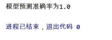
3.3 看一下结果—准确率
模型预测准确率为1.0,但是画树实在是有点复杂,接下来在Jupyter notebook上用sklearn库来实现决策树的图的绘制。
3.4 再是画图部分的代码
#导入相应的包
from sklearn import tree
from sklearn.tree import DecisionTreeClassifier
import graphviz
#先创建1个空的DataFrame
empty = pd.DataFrame(columns={'age':'','prescript':'','astigmatic':'','tearRate':''},index=range(24))
#将 Xtrain的所有  标称值 转换为 数值型
#不然它无法判断,它是自己根据数据的大小来选定一个中间值进行划分的
xlabel = ['age','prescript','astigmatic','tearRate'] # 4个特征
Xtrain = pd.DataFrame(columns={'age':'','prescript':'','astigmatic':'','tearRate':''},index=range(24)) #先创建一个空的dataframe,大小为24行,4列。方便后面加入转换好的数据。
for i in range(4): #0 1 2 3
    Xtrain1 = dataSet.iloc[:,i]
    labels = Xtrain1.unique().tolist()
    Xtrain1 = Xtrain1.apply(lambda x: labels.index(x)) #将本文转换为数字
    Xtrain[xlabel[i]]=Xtrain1 #对应的列  加入对应转换好的数值
#标签
Ytrain = dataSet.iloc[:,-1]
labels = Ytrain.unique().tolist()
Ytrain = Ytrain.apply(lambda x: labels.index(x)) #将本文转换为数字

#这是绘制 简单的 没颜色的 方的 树模型
clf = DecisionTreeClassifier()
clf = clf.fit(Xtrain, Ytrain)
tree.export_graphviz(clf)

#给图形增加标签和颜色,而且换成了圆形的框
dot_data = tree.export_graphviz(clf, out_file=None,
                                feature_names=['age','prescript','astigmatic','tearRate'],
                                class_names=['no lenses', 'soft','hard'],
                                filled=True, rounded=True,
                                special_characters=True)
graphviz.Source(dot_data)
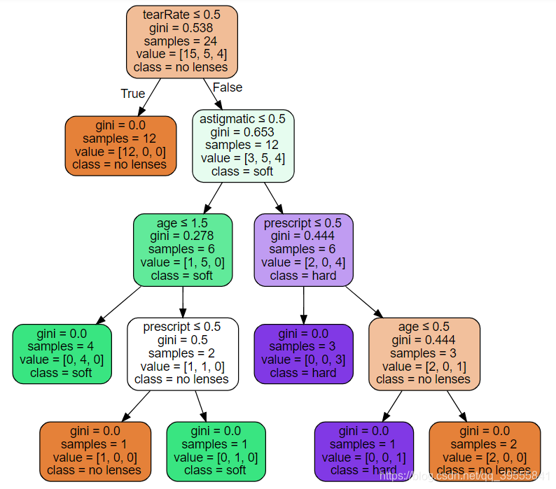
3.5 话不多说,上图。
先是普通版:

再是VIP版决策树的图:(分支都是左边Ture,右边False)
四、总结
4.1 决策树有点分类得太好了,就是过拟合了,因为那个预测都100%了,其实还需要剪枝,这个在第九章树回归了。
4.2 sep=’\t’可以用于Tab分隔符的数据。
4.3 决策树的构造算法有很多很多,最流行的是C4.5和CART,不同算法的分类依据也不同,这里用的是信息增益,信息增益越大的,熵减小的速度就越快,本书第9章讨论回归问题时将介绍CART算法,CART用的就是基尼不纯度了,越小越好,gini=0的就是最纯的。
4.4 熵,以前高中化学讲过,其实就是表示混乱程度用的,熵越大,越混乱,熵越小,越纯净,没杂质。
4.5 多写几个子函数,更方便点。
4.6 决策树模型生成后一定要及时保存,不然下一次再生成,如果数据多的话,会很浪费时间的。下次要用就直接load就行了。
4.7 其实一开始是在Jupyter notebook上写的,那个方便看结果,全部写好后,再去pycharm上封装起来,方便以后的使用。
4.8 两种方法: 用列表和字典创建空数据框
df = pd.DataFrame(data=None,columns=range(0,3),index=[0,1,2])
或者
df = pd.DataFrame(columns={‘qqq’:"",‘www’:""},index=[0,1])
4.9 谢谢阅读,我是刚学不久的小白,有错误的话欢迎各位大佬提出来,共同进步,谢谢了。


 1520
1520


 被折叠的 条评论
为什么被折叠?
被折叠的 条评论
为什么被折叠?
 到【灌水乐园】发言


