RNN、LSTM、GRU

RNN

recurrent neural network， 循环神经网络更多应用于序列数据的处理中，网络参数共享是RNN的一个重要特点。
RNN结构示意图如下：

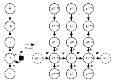
下面我们以具体的应用场景进行展开描述。

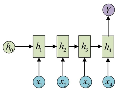
例如在文本分类问题中，输入的一句话可以看作是一个序列，输出为该条语句的类别标签。此时，RNN 的网络结构为：

其中，$x_i$表示语句中的一个单词，输出Y为类别标签。下面我们来看隐藏层单元中的运算，$h_i$表示了每一个隐层单元的状态：
$h_i=\varphi (W_h{h}_{i-1}+W_x{x}_i+b)$,
$W_x$是权重矩阵，$W_h$是状态转移矩阵, $\varphi$表示激活函数，可以选择$tanh$或者$ReLU$作为激活函数，上面模型最终的输出为:
$\hat{y}=\sigma (h_4)$,
$\sigma$也是激活函数，分类问题中，可以选择$sigmoid$函数作为激活函数。

关于模型的训练过程：
在RNN中，我们将梯度反向传播的过程叫做基于时间的反向传播算法。我们将损失函数记为$L(\hat{y},y)$, 我们要优化的参数是$W_x$和$W_h$, $h_4$时刻的输出的损失函数对$W_x$求偏导数，记为：
$\frac{\partial L_4}{\partial W_x}=\frac{\partial L_4}{\partial h_4}\frac{\partial h_4}{\partial W_x}+\frac{\partial L_4}{\partial h_4}\frac{\partial h_4}{\partial h_3}\frac{\partial h_3}{\partial W_x}+\frac{\partial L_4}{\partial h_4}\frac{\partial h_4}{\partial h_3}\frac{\partial h_3}{\partial h_2}\frac{\partial h_2}{\partial W_x}+\frac{\partial L_4}{\partial h_4}\frac{\partial h_4}{\partial h_3}\frac{\partial h_3}{\partial h_2}\frac{\partial h_2}{\partial h_1}\frac{\partial h_1}{\partial W_x}$
$h_4$时刻的输出的损失函数对$W_h$求偏导数，记为：
$\frac{\partial L_4}{\partial W_h}=\frac{\partial L_4}{\partial h_4}\frac{\partial h_4}{\partial W_h}+\frac{\partial L_4}{\partial h_4}\frac{\partial h_4}{\partial h_3}\frac{\partial h_3}{\partial W_h}+\frac{\partial L_4}{\partial h_4}\frac{\partial h_4}{\partial h_3}\frac{\partial h_3}{\partial h_2}\frac{\partial h_2}{\partial W_h}+\frac{\partial L_4}{\partial h_4}\frac{\partial h_4}{\partial h_3}\frac{\partial h_3}{\partial h_2}\frac{\partial h_2}{\partial h_1}\frac{\partial h_1}{\partial W_h}$
由此可见，对$W_x$和$W_h$求偏导均存在累乘项，即长期依赖问题，进而导致梯度消失或梯度爆炸问题。
任意$t$时刻计算损失函数对$W_x$和$W_h$的偏导数可以总结为：
$\frac{\partial L_t}{\partial W_x}={\sum }_{i=1}^t\frac{\partial L_t}{\partial h_t}({\prod }_{j=i+1}^t\frac{\partial h_j}{\partial h_{j-1}})\frac{\partial h_i}{\partial W_x}$

$\frac{\partial L_t}{\partial W_h}={\sum }_{i=1}^t\frac{\partial L_t}{\partial h_t}({\prod }_{j=i+1}^t\frac{\partial h_j}{\partial h_{j-1}})\frac{\partial h_i}{\partial W_h}$

由此，我们可以看到，RNN损失函数对参数的偏导数都存在下面项：
$\frac{\partial h_t}{\partial h_i}={\prod }_{j=i+1}^t\frac{\partial h_j}{\partial h_{j-1}}$
上面这个连乘是RNN梯度问题产生的根本原因。
RNN的目的是捕获长距离输入序列之间的依赖问题，但是由于存在梯度消失的问题，使得这一目标往往并不能取得很好的效果。

由于对$W_x$和$W_h$求偏导均存在长期依赖问题，这导致RNN在模型训练过程中很容易产生梯度消失或者梯度爆炸的问题，其中梯度消失问题更为棘手，因为梯度爆炸问题可以通过梯度裁剪，在一定程度上进行缓解，而梯度消失问题，往往需要从模型本身的结构上进行改进。在卷积神经网络中，为了缓解梯度消失问题，可以在网络结构中引入残差单元，通过残差学习的方式缓解梯度消失问题，而在循环神经网络中，LSTM和GRU对RNN结构的改进，在一定程度上缓解了RNN的梯度消失问题。

在介绍LSTM之前，我们补充介绍RNN网络的另外几种典型的应用场景：
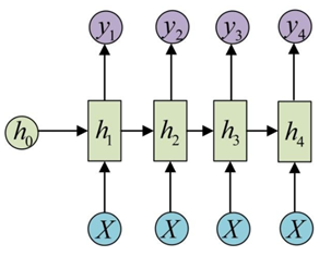
词性标注问题，对语句中的每一个单词进行词性标准，网络输入输出为N-N，网络结构如下：

机器翻译问题，将一种语言翻译到另外一种语言，模型的输入输出为N-M，网络结构如下图所示：

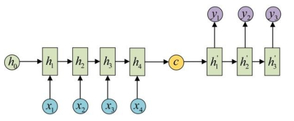
上面这种网络结构表示序列到序列的模型，也叫做Seq2Seq或者Encoder-Decoder模型，模型的左半部分表示编码器（Encoder），右半部分表示解码器（Decoder）。

LSTM

long short-term memory，长短期记忆网络是RNN的一种变体，它对RNN的隐藏状态单元的结构进行了改进，一定程度上缓解了梯度消失的问题（不能说是完全解决梯度消失问题）。

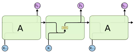
下面这张图表示的是一个标准的RNN单元：

然后，我们再来看LSTM的基本单元：

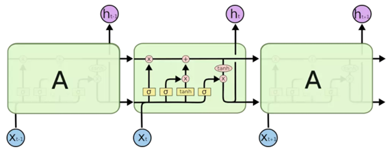
上面图中，$\sigma$ 和 $tanh$ 分别表示激活函数 $sigmoid(x)$ 和 $tanh(x)$ ，$sigmoid(x)$ 用于进行选择操作，$tanh(x)$ 用于进行变换操作，具体解释下面会进行介绍，粉色圆圈分别表示加法和乘法操作。

观察上面两张图，我们可以发现，LSTM的基本单元要比RNN复杂很多，下面，我们对LSTM基本单元中的每一个部分进行详细的介绍。LSTM基本单元我们称作细胞（Cell），每个 cell 中有三个输入，分别是t时刻的输入，上一个 cell 的状态$C_{t-1}$，以及上一个 cell 的输出。另外，每个Cell中包含有三个门控单元，从左到右，依次分别叫做遗忘门，输入门和和输出门，每一个门的输入都由前一个时刻的状态$h_{t-1}$和当前时刻的输入$x_t$共同组成：$[h_{t-1},x_t]$,

遗忘门
$t$ 时刻遗忘门(forget)得到的输出为：
$f(t)=\sigma (W_f[h_{t-1},x_t]+b_f)=\sigma (W_{fh}{h}_{t-1}+W_{fx}{x}_{t-1}+b_f)$
输入门
$t$ 时刻输入门(input)得到的输出为：
$i(t)=\sigma (W_i[h_{t-1},x_t]+b_i)=\sigma (W_{ih}{h}_{t-1}+W_{ix}{x}_{t-1}+b_i)$
同时有：
$\widetilde{c_t}=tanh(W_c[h_{t-1},x_t]+b_c)=tanh(W_{ch}{h}_{t-1}+W_{cx}{x}_{t-1}+b_c)$
输出门
$t$ 时刻输出门(output)得到的输出为：
$o(t)=\sigma (W_o[h_{t-1},x_t]+b_o)=\sigma (W_{oh}{h}_{t-1}+W_{ox}{x}_{t-1}+b_o)$

在得到 cell 内部的计算流程的输出之后，我们就可以得到了每个 cell 的两个输出：当前 cell 的状态 $C_t$ 和 当前 cell 的输出$h_t$,分别是：
$c_t=c_{t-1}\ast f_t+i_t\ast \widetilde{c_t}$
$h_t=tanh(c_t)\ast o_t$
我们可以将$c_t$和$h_t$理解为每个cell的两个状态变量，LSTM相对标准RNN，其内部的运算机制要复杂很多，为了减小计算复杂度，GRU针对LSTM进行了改进，使每个cell中只有一个状态量，一定程度上减少了计算复杂度。另外一点值得注意的是，在RNN中，每个cell只有一个状态变量$h_t$，在LSTM中与之相对应的是$c_t$,而不是$h_t$, 这在上面RNN和LSTM基本单元的结构对比图中也可以体现出来，并且，cell 的输出是基于$h_t$得到的，这也是需要注意的。

介绍完LSTM的三个门控单元的基本操作原理之后，那么LSTM具体在训练中是怎么缓解梯度消失问题的呢？我们先看LSTM的训练过程。
在LSTM的训练过程中，我们需要更新的参数有$W_f$, $W_i$, $W_c$ 和 $W_o$,
记 t 时刻的损失函数为 $L_t$, 我们先看损失函数对参数$W_c$的偏导数：
$\frac{\partial L_t}{\partial W_c}=\frac{\partial L_t}{\partial h_t}\frac{\partial h_t}{\partial c_t}\frac{\partial \widetilde{c_t}}{\partial W_c}+\frac{\partial L_t}{\partial h_t}\frac{\partial h_t}{\partial c_t}\frac{\partial \widetilde{c_t}}{\partial c_{t-1}}\frac{\partial c_{t-1}}{\partial {\tilde{c}}_{t-1}}\frac{\partial {\tilde{c}}_{t-1}}{\partial W_c}+......$
从上面的公式来看，我们LSTM的求导过程还是很复杂的，我们试图直接从中分析出是否存在梯度问题比较不容易。

但是，前面我们说到，RNN中，$\frac{\partial h_t}{\partial h_i}$是一个连乘，是产生梯度问题的根本原因，并且RNN中$h_i$的传递关系为：
$h_i=\varphi (W_h{h}_{i-1}+W_x{x}_i+b)$
另外RNN中：$\frac{\partial h_t}{\partial h_{t-1}}=\frac{\partial h_t}{\partial h_{t-1}}$

我们前面还说到，LSTM中的$c_i$对应了RNN中的$h_i$,并且 $c_i$ 的在每个 cell 中的传递关系为：
$c_t=c_{t-1}\ast f_t+i_t\ast \widetilde{c_t}$
进一步，我们再看 $\frac{\partial c_t}{\partial c_i}$ 的计算, 更简单的，我们先看$\frac{\partial c_t}{\partial c_{t-1}}$的计算，计算这个偏导数之前，我们需要注意， $f_t$, $i_t$, ${\tilde{c}}_t$的计算都是含有$h_{t-1}$的，而$h_{t-1}$的计算又是包含$c_{t-1}$的，因此，$f_t$, $i_t$, ${\tilde{c}}_t$都是$c_{t-1}$的复合函数。
$\frac{\partial c_t}{\partial c_{t-1}}=f_t+\frac{\partial f_t}{\partial c_{t-1}}\ast c_{t-1}+\frac{\partial i_t}{\partial c_{t-1}}\ast \widetilde{c_t}+i_t\ast \frac{\widetilde{c_t}}{\partial c_{t-1}}$
由此，我们看到LSTM中的状态计算$\frac{\partial c_t}{\partial c_{t-1}}$ 与RNN中的状态计算$\frac{\partial h_t}{\partial h_{t-1}}$有明显的不同。
再回到LSTM中的$\frac{\partial c_t}{\partial c_{t-1}}$，这项偏导数的第一项是$f_t$，而$f_t$是遗忘门 forget gate 的输出，而forget gate 的输出 $f_t$ 是经过 sigmoid 函数得到的，若输出$f_t$的值是1，则完全保留旧状态，若输出$f_t$的值是0，则完全舍弃旧状态。当$f_t$的值为1或者接近1时，$\frac{\partial c_t}{\partial c_{t-1}}$就存在梯度了，这就缓解了梯度消失的问题。

我们讲，LSTM能够缓解RNN的梯度消失问题，就是因为$c_t$到$c_{t-1}$这条路径上的梯度信息得到了缓解，在其他路径上的梯度信息并没有得到缓解，另外，遗忘门的作用就是保留前一个cell的状态信息，这也就解决了RNN中的长距离依赖问题。

GRU

由于LSTM的 cell 内部结构较为复杂，GRU可以理解为对LSTM的简化，其内部结构对于前一个状态信息的取舍也是通过门控单元来实现的。