


AdaBoost
将多个单模型组合成一个综合模型的方式早已成为现代机器学习模型采用的主流方法。
AdaBoost正是集成学习中Boosting框架的一种经典代表。
Boosting
Boosting是机器学习中的一种集成学习框架。
之前的学习的模型都称作单模型,也称弱分类器。而集成学习的意思是将多个弱分类器组合成一个强分类器,这个强分类器能取所有弱分类器之所长,达到相对的最优性能
Boosting算法的一般过程如下。以分类问题为例,给定一个训练集,训练弱分类器要比训练强分类器容易很多,从第一个弱分类器开始,Boosting通过训练多个弱分类器,并在训练过程中不断改变训练样本的概率分布,使得每次训练时算法都会更加关注上一个弱分类器的错误。通过组合多个这样的弱分类器,便可以获得一个近乎完美的强分类器。
AdaBoost基本原理
AdaBoost的全称为Adaptive Boosting,可以翻译为自适应提升算法。
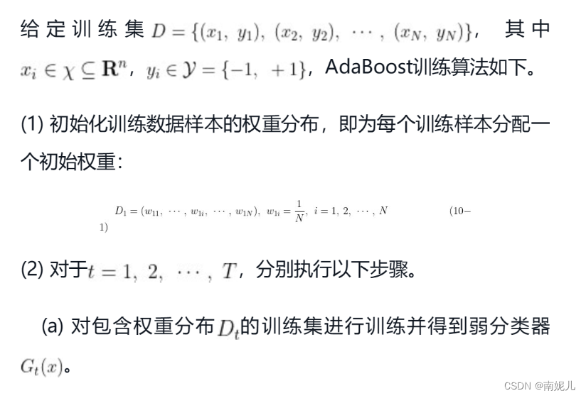
AdaBoost是一种通过改变训练样本权重来学习多个弱分类器并线性组合成强分类器的Boosting算法。
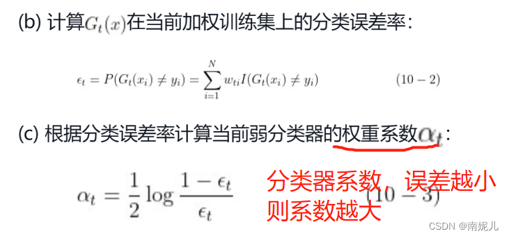
一般来说,Boosting方法要解答两个关键问题:一是在训练过程中如何改变训练样本的权重或者概率分布,二是如何将多个弱分类器组合成一个强分类器。针对这两个问题,AdaBoost的做法非常朴素,一是提高前一轮被弱分类器分类错误的样本的权重,而降低分类正确的样本的权重;二是对多个弱分类器进行线性组合,提高分类效果好的弱分类器的权重,降低分类误差率高的弱分类器的权重。


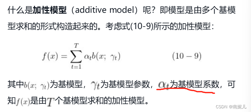
加性模型
AdaBoost是以加性模型为模型、指数函数为损失函数、前向分步为算法的分类学习算法。

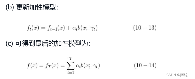
针对这样一个较为复杂的优化问题,可以采用前向分步算法进行求解。其基本思路如下:针对加性模型的特点,从前往后每次只优化一个基模型的参数
每一步优化的表达式:

优化步骤:

numpy代码实现
import numpy as np
import pandas as pd
import matplotlib.pyplot as plt

from sklearn.model_selection import train_test_split
# 导入sklearn模拟二分类数据生成模块
from sklearn.datasets import make_blobs
# 生成模拟二分类数据集
X, y =  make_blobs(n_samples=150, n_features=2, centers=2,
  cluster_std=1.2, random_state=40)

# 将标签转换为1/-1
y_ = y.copy()
y_[y_==0] = -1
y_ = y_.astype(float)
# 训练/测试数据集划分
X_train, X_test, y_train, y_test = train_test_split(X, y_,
 test_size=0.3, random_state=43)
# 设置颜色参数
colors = {0:'r', 1:'g'}
# 绘制二分类数据集的散点图
plt.scatter(X[:,0], X[:,1], marker='o', c=pd.Series(y).map(colors))
plt.show()

### 定义决策树桩类
### 作为Adaboost弱分类器
class DecisionStump():
    def __init__(self):
        # 基于划分阈值决定样本分类为1还是-1
        self.label = 1
        # 特征索引
        self.feature_index = None
        # 特征划分阈值
        self.threshold = None
        # 指示分类准确率的值
        self.alpha = None

### 定义AdaBoost算法类
class Adaboost:
    # 弱分类器个数
    def __init__(self, n_estimators=5):
        self.n_estimators = n_estimators

    # Adaboost拟合算法
    def fit(self, X, y):
        m, n = X.shape
        # (1)初始化权重分布为均匀分布 1/N
        w = np.full(m, (1 / m))
        # 处初始化基分类器列表
        self.estimators = []
        # (2) for m in (1,2,...,M)
        for _ in range(self.n_estimators):
            # 定义一个弱分类器
            estimator = DecisionStump()
            # 设定一个最小化误差
            min_error = float('inf')
            # 遍历数据集特征,根据最小分类误差率选择最优划分特征
            for i in range(n):
                # 获取特征值
                values = np.expand_dims(X[:, i], axis=1)
                # 特征取值去重
                unique_values = np.unique(values)
                # 尝试将每一个特征值作为分类阈值
                for threshold in unique_values:
                    p = 1
                    # 初始化所有预测值为1
                    pred = np.ones(np.shape(y))
                    # 小于分类阈值的预测值为-1
                    pred[X[:, i] < threshold] = -1
                    # 2.b 计算误差率
                    error = sum(w[y != pred])

                    # 如果分类误差大于0.5,则进行正负预测翻转
                    # 例如 error = 0.6 => (1 - error) = 0.4
                    if error > 0.5:
                        error = 1 - error
                        p = -1

                    # 一旦获得最小误差则保存相关参数配置
                    if error < min_error:
                        estimator.label = p
                        estimator.threshold = threshold
                        estimator.feature_index = i
                        min_error = error

            # 2.c 计算基分类器的权重
            estimator.alpha = 0.5 * np.log((1.0 - min_error) / (min_error + 1e-9))
            # 初始化所有预测值为1
            preds = np.ones(np.shape(y))
            # 获取所有小于阈值的负类索引
            negative_idx = (estimator.label * X[:, estimator.feature_index] < estimator.label * estimator.threshold)
            # 将负类设为 '-1'
            preds[negative_idx] = -1
            # 2.d 更新样本权重
            w *= np.exp(-estimator.alpha * y * preds)
            w /= np.sum(w)

            # 保存该弱分类器
            self.estimators.append(estimator)

    # 定义预测函数
    def predict(self, X):
        m = len(X)
        y_pred = np.zeros((m, 1))
        # 计算每个弱分类器的预测值
        for estimator in self.estimators:
            # 初始化所有预测值为1
            predictions = np.ones(np.shape(y_pred))
            # 获取所有小于阈值的负类索引
            negative_idx = (estimator.label * X[:, estimator.feature_index] < estimator.label * estimator.threshold)
            # 将负类设为 '-1'
            predictions[negative_idx] = -1
            # 2.e 对每个弱分类器的预测结果进行加权
            y_pred += estimator.alpha * predictions

        # 返回最终预测结果
        y_pred = np.sign(y_pred).flatten()
        return y_pred

# 导入sklearn准确率计算函数
from sklearn.metrics import accuracy_score
# 创建Adaboost模型实例
clf = Adaboost(n_estimators=5)
# 模型拟合
clf.fit(X_train, y_train)
# 模型预测
y_pred = clf.predict(X_test)
# 计算模型预测准确率
accuracy = accuracy_score(y_test, y_pred)
print("Accuracy of AdaBoost by numpy:", accuracy)
sklearn代码实现
import numpy as np
import pandas as pd
import matplotlib.pyplot as plt

from sklearn.model_selection import train_test_split
# 导入sklearn模拟二分类数据生成模块
from sklearn.datasets import make_blobs
# 生成模拟二分类数据集
X, y =  make_blobs(n_samples=1500, n_features=4, centers=2,
  cluster_std=1.2, random_state=40)

# 训练/测试数据集划分
X_train, X_test, y_train, y_test = train_test_split(X, y,
 test_size=0.3, random_state=43)
# 设置颜色参数
colors = {0:'r', 1:'g'}
# 绘制二分类数据集的散点图
plt.scatter(X[:,0], X[:,1], marker='o', c=pd.Series(y).map(colors))
plt.show()

# 导入sklearn adaboost分类器
from sklearn.metrics import accuracy_score
from sklearn.ensemble import AdaBoostClassifier
# 创建Adaboost模型实例
clf_ = AdaBoostClassifier(n_estimators=5, random_state=0)
# 模型拟合
clf_.fit(X_train, y_train)
# 模型预测
y_pred_ = clf_.predict(X_test)
# 计算模型预测准确率
accuracy = accuracy_score(y_test, y_pred_)
print("Accuracy of AdaBoost by sklearn:", accuracy)
GBDT
虽然AdaBoost是集成学习Boosting框架的经典模型,但目前工业界应用更广泛是GBDT系列模型。从集成学习的范式上来看,GBDT仍属于Boosting框架。
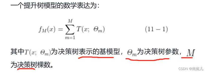
提升树
在AdaBoost中,我们可以使用任意单模型作为弱分类器,但提升树的弱分类器只能是决策树模型。
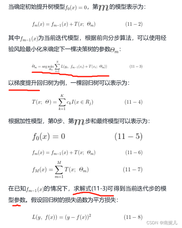
针对提升树模型,加性模型和前向分步算法的组合是典型的求解方式。当损失函数为平方损失和指数损失时,前向分步算法的每一步迭代都较为容易求解,但如果是一般的损失函数,前向分步算法的每一步迭代并不容易。所以,有研究提出使用损失函数的负梯度在当前模型的值来求解更为一般的提升树模型。这种基于负梯度求解提升树前向分步迭代过程的方法也叫梯度提升树。
GBDT算法的原理推导
GBDT的全称为梯度提升决策树(gradient boosting decision tree),其基模型(弱分类器)为CART决策树,针对分类问题的基模型为二叉分类树,对应梯度提升模型就叫GBDT;针对回归问题的基模型为二叉回归树,对应的梯度提升模型叫作GBRT(gradient boosting regression tree)。


一般步骤:

numpy代码实现
cart.py
import numpy as np
from utils import feature_split, calculate_gini

### 定义树结点
class TreeNode():
    def __init__(self, feature_i=None, threshold=None,
               leaf_value=None, left_branch=None, right_branch=None):
        # 特征索引
        self.feature_i = feature_i
        # 特征划分阈值
        self.threshold = threshold
        # 叶子节点取值
        self.leaf_value = leaf_value
        # 左子树
        self.left_branch = left_branch
        # 右子树
        self.right_branch = right_branch


### 定义二叉决策树
class BinaryDecisionTree(object):
    ### 决策树初始参数
    def __init__(self, min_samples_split=2, min_gini_impurity=999,
                 max_depth=float("inf"), loss=None):
        # 根结点
        self.root = None
        # 节点最小分裂样本数
        self.min_samples_split = min_samples_split
        # 节点初始化基尼不纯度
        self.mini_gini_impurity = min_gini_impurity
        # 树最大深度
        self.max_depth = max_depth
        # 基尼不纯度计算函数
        self.gini_impurity_calculation = None
        # 叶子节点值预测函数
        self._leaf_value_calculation = None
        # 损失函数
        self.loss = loss

    ### 决策树拟合函数
    def fit(self, X, y, loss=None):
        # 递归构建决策树
        self.root = self._build_tree(X, y)
        self.loss=None

    ### 决策树构建函数
    def _build_tree(self, X, y, current_depth=0):
        # 初始化最小基尼不纯度
        init_gini_impurity = 999
        # 初始化最佳特征索引和阈值
        best_criteria = None
        # 初始化数据子集
        best_sets = None

        if len(np.shape(y)) == 1:
            y = np.expand_dims(y, axis=1)

        # 合并输入和标签
        Xy = np.concatenate((X, y), axis=1)
        # 获取样本数和特征数
        n_samples, n_features = X.shape
        # 设定决策树构建条件
        # 训练样本数量大于节点最小分裂样本数且当前树深度小于最大深度
        if n_samples >= self.min_samples_split and current_depth <= self.max_depth:
            # 遍历计算每个特征的基尼不纯度
            for feature_i in range(n_features):
                # 获取第i特征的所有取值
                feature_values = np.expand_dims(X[:, feature_i], axis=1)
                # 获取第i个特征的唯一取值
                unique_values = np.unique(feature_values)

                # 遍历取值并寻找最佳特征分裂阈值
                for threshold in unique_values:
                    # 特征节点二叉分裂
                    Xy1, Xy2 = feature_split(Xy, feature_i, threshold)
                    # 如果分裂后的子集大小都不为0
                    if len(Xy1) > 0 and len(Xy2) > 0:
                        # 获取两个子集的标签值
                        y1 = Xy1[:, n_features:]
                        y2 = Xy2[:, n_features:]

                        # 计算基尼不纯度
                        impurity = self.impurity_calculation(y, y1, y2)

                        # 获取最小基尼不纯度
                        # 最佳特征索引和分裂阈值
                        if impurity < init_gini_impurity:
                            init_gini_impurity = impurity
                            best_criteria = {"feature_i": feature_i, "threshold": threshold}
                            best_sets = {
                                "leftX": Xy1[:, :n_features],
                                "lefty": Xy1[:, n_features:],
                                "rightX": Xy2[:, :n_features],
                                "righty": Xy2[:, n_features:]
                                }

        # 如果计算的最小不纯度小于设定的最小不纯度
        if init_gini_impurity < self.mini_gini_impurity:
            # 分别构建左右子树
            left_branch = self._build_tree(best_sets["leftX"], best_sets["lefty"], current_depth + 1)
            right_branch = self._build_tree(best_sets["rightX"], best_sets["righty"], current_depth + 1)
            return TreeNode(feature_i=best_criteria["feature_i"], threshold=best_criteria["threshold"], left_branch=left_branch, right_branch=right_branch)

        # 计算叶子计算取值
        leaf_value = self._leaf_value_calculation(y)
        return TreeNode(leaf_value=leaf_value)

    ### 定义二叉树值预测函数
    def predict_value(self, x, tree=None):
        if tree is None:
            tree = self.root
        # 如果叶子节点已有值,则直接返回已有值
        if tree.leaf_value is not None:
            return tree.leaf_value
        # 选择特征并获取特征值
        feature_value = x[tree.feature_i]
        # 判断落入左子树还是右子树
        branch = tree.right_branch
        if isinstance(feature_value, int) or isinstance(feature_value, float):
            if feature_value >= tree.threshold:
                branch = tree.left_branch
        elif feature_value == tree.threshold:
            branch = tree.right_branch
        # 测试子集
        return self.predict_value(x, branch)

    ### 数据集预测函数
    def predict(self, X):
        y_pred = [self.predict_value(sample) for sample in X]
        return y_pred

# CART分类树
class ClassificationTree(BinaryDecisionTree):
    ### 定义基尼不纯度计算过程
    def _calculate_gini_impurity(self, y, y1, y2):
        p = len(y1) / len(y)
        gini = calculate_gini(y)
	# 基尼不纯度
        gini_impurity = p * calculate_gini(y1) + (1-p) * calculate_gini(y2)
        return gini_impurity

    ### 多数投票
    def _majority_vote(self, y):
        most_common = None
        max_count = 0
        for label in np.unique(y):
            # 统计多数
            count = len(y[y == label])
            if count > max_count:
                most_common = label
                max_count = count
        return most_common

    # 分类树拟合
    def fit(self, X, y):
        self.impurity_calculation = self._calculate_gini_impurity
        self._leaf_value_calculation = self._majority_vote
        super(ClassificationTree, self).fit(X, y)


### CART回归树
class RegressionTree(BinaryDecisionTree):
	# 计算方差减少量
    def _calculate_variance_reduction(self, y, y1, y2):
        var_tot = np.var(y, axis=0)
        var_y1 = np.var(y1, axis=0)
        var_y2 = np.var(y2, axis=0)
        frac_1 = len(y1) / len(y)
        frac_2 = len(y2) / len(y)
        # 计算方差减少量
        variance_reduction = var_tot - (frac_1 * var_y1 + frac_2 * var_y2)
        return sum(variance_reduction)

    # 节点值取平均
    def _mean_of_y(self, y):
        value = np.mean(y, axis=0)
        return value if len(value) > 1 else value[0]

    # 回归树拟合
    def fit(self, X, y):
        self.impurity_calculation = self._calculate_variance_reduction
        self._leaf_value_calculation = self._mean_of_y
        super(RegressionTree, self).fit(X, y)
utils.py
import numpy as np

### 定义二叉特征分裂函数
def feature_split(X, feature_i, threshold):
    split_func = None
    if isinstance(threshold, int) or isinstance(threshold, float):
        split_func = lambda sample: sample[feature_i] >= threshold
    else:
        split_func = lambda sample: sample[feature_i] == threshold

    X_left = np.array([sample for sample in X if split_func(sample)])
    X_right = np.array([sample for sample in X if not split_func(sample)])

    return np.array([X_left, X_right])


### 计算基尼指数
def calculate_gini(y):
    y = y.tolist()
    probs = [y.count(i)/len(y) for i in np.unique(y)]
    gini = sum([p*(1-p) for p in probs])
    return gini


### 打乱数据
def data_shuffle(X, y, seed=None):
    if seed:
        np.random.seed(seed)
    idx = np.arange(X.shape[0])
    np.random.shuffle(idx)
    return X[idx], y[idx]
import numpy as np
from cart import TreeNode, BinaryDecisionTree, ClassificationTree, RegressionTree
from sklearn.model_selection import train_test_split
from sklearn.metrics import mean_squared_error
from utils import feature_split, calculate_gini, data_shuffle


### GBDT定义
class GBDT(object):
    def __init__(self, n_estimators, learning_rate, min_samples_split,
                 min_gini_impurity, max_depth, regression):
        ### 常用超参数
        # 树的棵树
        self.n_estimators = n_estimators
        # 学习率
        self.learning_rate = learning_rate
        # 结点最小分裂样本数
        self.min_samples_split = min_samples_split
        # 结点最小基尼不纯度
        self.min_gini_impurity = min_gini_impurity
        # 最大深度
        self.max_depth = max_depth
        # 默认为回归树
        self.regression = regression
        # 损失为平方损失
        self.loss = SquareLoss()
        # 如果是分类树,需要定义分类树损失函数
        # 这里省略,如需使用,需自定义分类损失函数
        if not self.regression:
            self.loss = None
        # 多棵树叠加
        self.estimators = []
        for i in range(self.n_estimators):
            self.estimators.append(RegressionTree(min_samples_split=self.min_samples_split,
                                                  min_gini_impurity=self.min_gini_impurity,
                                                  max_depth=self.max_depth))

    # 拟合方法
    def fit(self, X, y):
        # 前向分步模型初始化,第一棵树
        self.estimators[0].fit(X, y)
        # 第一棵树的预测结果
        y_pred = self.estimators[0].predict(X)
        # 前向分步迭代训练
        for i in range(1, self.n_estimators):
            gradient = self.loss.gradient(y, y_pred)
            self.estimators[i].fit(X, gradient)
            y_pred -= np.multiply(self.learning_rate, self.estimators[i].predict(X))

    # 预测方法
    def predict(self, X):
        # 回归树预测
        y_pred = self.estimators[0].predict(X)
        for i in range(1, self.n_estimators):
            y_pred -= np.multiply(self.learning_rate, self.estimators[i].predict(X))
        # 分类树预测
        if not self.regression:
            # 将预测值转化为概率
            y_pred = np.exp(y_pred) / np.expand_dims(np.sum(np.exp(y_pred), axis=1), axis=1)
            # 转化为预测标签
            y_pred = np.argmax(y_pred, axis=1)
        return y_pred


### GBDT分类树
class GBDTClassifier(GBDT):
    def __init__(self, n_estimators=200, learning_rate=.5, min_samples_split=2,
                 min_info_gain=1e-6, max_depth=2):
        super(GBDTClassifier, self).__init__(n_estimators=n_estimators,
                                             learning_rate=learning_rate,
                                             min_samples_split=min_samples_split,
                                             min_gini_impurity=min_info_gain,
                                             max_depth=max_depth,
                                             regression=False)

    # 拟合方法
    def fit(self, X, y):
        super(GBDTClassifier, self).fit(X, y)


### GBDT回归树
class GBDTRegressor(GBDT):
    def __init__(self, n_estimators=300, learning_rate=0.1, min_samples_split=2,
                 min_var_reduction=1e-6, max_depth=3):
        super(GBDTRegressor, self).__init__(n_estimators=n_estimators,
                                            learning_rate=learning_rate,
                                            min_samples_split=min_samples_split,
                                            min_gini_impurity=min_var_reduction,
                                            max_depth=max_depth,
                                            regression=True)

### 定义回归树的平方损失
class SquareLoss():
    # 定义平方损失
    def loss(self, y, y_pred):
        return 0.5 * np.power((y - y_pred), 2)
    # 定义平方损失的梯度
    def gradient(self, y, y_pred):
        return -(y - y_pred)

### GBDT分类树
# 导入sklearn数据集模块
from sklearn import datasets
# 导入波士顿房价数据集
boston = datasets.load_boston()
# 打乱数据集
X, y = data_shuffle(boston.data, boston.target, seed=13)
X = X.astype(np.float32)
offset = int(X.shape[0] * 0.9)
# 划分数据集
X_train, X_test, y_train, y_test = train_test_split(X, y, test_size=0.9)
# 创建GBRT实例
model = GBDTRegressor()
# 模型训练
model.fit(X_train, y_train)
# 模型预测
y_pred = model.predict(X_test)
# 计算模型预测的均方误差
mse = mean_squared_error(y_test, y_pred)
print ("Mean Squared Error of NumPy GBRT:", mse)
sklearn代码实现
# 导入sklearn数据集模块
import sklearn
from sklearn import datasets
import numpy as np
from sklearn.model_selection import train_test_split
from sklearn.metrics import mean_squared_error
# 导入波士顿房价数据集
boston = datasets.load_boston()
# 打乱数据集
X, y = sklearn.utils.shuffle(boston.data, boston.target)
X = X.astype(np.float32)
offset = int(X.shape[0] * 0.9)
# 划分数据集
X_train, X_test, y_train, y_test = train_test_split(X, y, test_size=0.3)

# 导入sklearn GBDT模块
from sklearn.ensemble import GradientBoostingRegressor
from sklearn.metrics import r2_score
# 创建模型实例
reg = GradientBoostingRegressor(n_estimators=200, learning_rate=0.5,
                                 max_depth=4, random_state=0)
# 模型拟合
reg.fit(X_train, y_train)
# 模型预测
y_pred = reg.predict(X_test)
# 计算模型预测的均方误差
mse = mean_squared_error(y_test, y_pred)
print('相关系数',reg.score(X_test,y_test))
print('相关系数',r2_score(y_test,y_pred))
print ("Mean Squared Error of sklearn GBRT:", mse)
XGBoost
从算法精度、速度和泛化能力等性能指标来看GBDT,仍然有较大的优化空间。XGBoost正是一种基于GBDT的顶级梯度提升模型。相较于GBDT,XGBoost的最大特性在于对损失函数展开到二阶导数,使得梯度提升树模型更能逼近其真实损失
numpy代码实现
utils.py
import numpy as np

### 定义二叉特征分裂函数
def feature_split(X, feature_i, threshold):
    split_func = None
    if isinstance(threshold, int) or isinstance(threshold, float):
        split_func = lambda sample: sample[feature_i] >= threshold
    else:
        split_func = lambda sample: sample[feature_i] == threshold

    X_left = np.array([sample for sample in X if split_func(sample)])
    X_right = np.array([sample for sample in X if not split_func(sample)])
    return np.array([X_left, X_right])

### 计算基尼指数
def calculate_gini(y):
    y = y.tolist()
    probs = [y.count(i)/len(y) for i in np.unique(y)]
    gini = sum([p*(1-p) for p in probs])
    return gini

### 打乱数据
def data_shuffle(X, y, seed=None):
    if seed:
        np.random.seed(seed)
    idx = np.arange(X.shape[0])
    np.random.shuffle(idx)
    return X[idx], y[idx]

### 类别标签转换
def cat_label_convert(y, n_col=None):
    if not n_col:
        n_col = np.amax(y) + 1
    one_hot = np.zeros((y.shape[0], n_col))
    one_hot[np.arange(y.shape[0]), y] = 1
    return one_hot
cart.py
import numpy as np
from utils import feature_split, calculate_gini

### 定义树结点
class TreeNode():
    def __init__(self, feature_i=None, threshold=None,
               leaf_value=None, left_branch=None, right_branch=None):
        # 特征索引
        self.feature_i = feature_i
        # 特征划分阈值
        self.threshold = threshold
        # 叶子节点取值
        self.leaf_value = leaf_value
        # 左子树
        self.left_branch = left_branch
        # 右子树
        self.right_branch = right_branch

### 定义二叉决策树
class BinaryDecisionTree(object):
    ### 决策树初始参数
    def __init__(self, min_samples_split=2, min_gini_impurity=999,
                 max_depth=float("inf"), loss=None):
        # 根结点
        self.root = None
        # 节点最小分裂样本数
        self.min_samples_split = min_samples_split
        # 节点初始化基尼不纯度
        self.min_gini_impurity = min_gini_impurity
        # 树最大深度
        self.max_depth = max_depth
        # 基尼不纯度计算函数
        self.gini_impurity_calculation = None
        # 叶子节点值预测函数
        self._leaf_value_calculation = None
        # 损失函数
        self.loss = loss

    ### 决策树拟合函数
    def fit(self, X, y, loss=None):
        # 递归构建决策树
        self.root = self._build_tree(X, y)
        self.loss=None

    ### 决策树构建函数
    def _build_tree(self, X, y, current_depth=0):
        # 初始化最小基尼不纯度
        init_gini_impurity = 999
        # 初始化最佳特征索引和阈值
        best_criteria = None
        # 初始化数据子集
        best_sets = None

        if len(np.shape(y)) == 1:
            y = np.expand_dims(y, axis=1)

        # 合并输入和标签
        Xy = np.concatenate((X, y), axis=1)
        # 获取样本数和特征数
        n_samples, n_features = X.shape
        # 设定决策树构建条件
        # 训练样本数量大于节点最小分裂样本数且当前树深度小于最大深度
        if n_samples >= self.min_samples_split and current_depth <= self.max_depth:
            # 遍历计算每个特征的基尼不纯度
            for feature_i in range(n_features):
                # 获取第i特征的所有取值
                feature_values = np.expand_dims(X[:, feature_i], axis=1)
                # 获取第i个特征的唯一取值
                unique_values = np.unique(feature_values)

                # 遍历取值并寻找最佳特征分裂阈值
                for threshold in unique_values:
                    # 特征节点二叉分裂
                    Xy1, Xy2 = feature_split(Xy, feature_i, threshold)
                    # 如果分裂后的子集大小都不为0
                    if len(Xy1) > 0 and len(Xy2) > 0:
                        # 获取两个子集的标签值
                        y1 = Xy1[:, n_features:]
                        y2 = Xy2[:, n_features:]

                        # 计算基尼不纯度
                        impurity = self.impurity_calculation(y, y1, y2)

                        # 获取最小基尼不纯度
                        # 最佳特征索引和分裂阈值
                        if impurity < init_gini_impurity:
                            init_gini_impurity = impurity
                            best_criteria = {"feature_i": feature_i, "threshold": threshold}
                            best_sets = {
                                "leftX": Xy1[:, :n_features],
                                "lefty": Xy1[:, n_features:],
                                "rightX": Xy2[:, :n_features],
                                "righty": Xy2[:, n_features:]
                                }

        # 如果计算的最小不纯度小于设定的最小不纯度
        if init_gini_impurity < self.min_gini_impurity:
            # 分别构建左右子树
            left_branch = self._build_tree(best_sets["leftX"], best_sets["lefty"], current_depth + 1)
            right_branch = self._build_tree(best_sets["rightX"], best_sets["righty"], current_depth + 1)
            return TreeNode(feature_i=best_criteria["feature_i"], threshold=best_criteria["threshold"], left_branch=left_branch, right_branch=right_branch)

        # 计算叶子计算取值
        leaf_value = self._leaf_value_calculation(y)
        return TreeNode(leaf_value=leaf_value)

    ### 定义二叉树值预测函数
    def predict_value(self, x, tree=None):
        if tree is None:
            tree = self.root
        # 如果叶子节点已有值,则直接返回已有值
        if tree.leaf_value is not None:
            return tree.leaf_value
        # 选择特征并获取特征值
        feature_value = x[tree.feature_i]
        # 判断落入左子树还是右子树
        branch = tree.right_branch
        if isinstance(feature_value, int) or isinstance(feature_value, float):
            if feature_value >= tree.threshold:
                branch = tree.left_branch
        elif feature_value == tree.threshold:
            branch = tree.right_branch
        # 测试子集
        return self.predict_value(x, branch)

    ### 数据集预测函数
    def predict(self, X):
        y_pred = [self.predict_value(sample) for sample in X]
        return y_pred


class ClassificationTree(BinaryDecisionTree):
    ### 定义基尼不纯度计算过程
    def _calculate_gini_impurity(self, y, y1, y2):
        p = len(y1) / len(y)
        gini = calculate_gini(y)
        gini_impurity = p * calculate_gini(y1) + (1-p) * calculate_gini(y2)
        return gini_impurity

    ### 多数投票
    def _majority_vote(self, y):
        most_common = None
        max_count = 0
        for label in np.unique(y):
            # 统计多数
            count = len(y[y == label])
            if count > max_count:
                most_common = label
                max_count = count
        return most_common

    # 分类树拟合
    def fit(self, X, y):
        self.impurity_calculation = self._calculate_gini_impurity
        self._leaf_value_calculation = self._majority_vote
        super(ClassificationTree, self).fit(X, y)


### CART回归树
class RegressionTree(BinaryDecisionTree):
	# 计算方差减少量
    def _calculate_variance_reduction(self, y, y1, y2):
        var_tot = np.var(y, axis=0)
        var_y1 = np.var(y1, axis=0)
        var_y2 = np.var(y2, axis=0)
        frac_1 = len(y1) / len(y)
        frac_2 = len(y2) / len(y)
        # 计算方差减少量
        variance_reduction = var_tot - (frac_1 * var_y1 + frac_2 * var_y2)
        return sum(variance_reduction)

    # 节点值取平均
    def _mean_of_y(self, y):
        value = np.mean(y, axis=0)
        return value if len(value) > 1 else value[0]

	# 回归树拟合
    def fit(self, X, y):
        self.impurity_calculation = self._calculate_variance_reduction
        self._leaf_value_calculation = self._mean_of_y
        super(RegressionTree, self).fit(X, y)
import numpy as np
from cart import TreeNode, BinaryDecisionTree
from sklearn.model_selection import train_test_split
from sklearn.metrics import accuracy_score
from utils import cat_label_convert

### XGBoost单棵树类
class XGBoost_Single_Tree(BinaryDecisionTree):
    # 结点分裂方法
    def node_split(self, y):
        # 中间特征所在列
        feature = int(np.shape(y)[1]/2)
        # 左子树为真实值,右子树为预测值
        y_true, y_pred = y[:, :feature], y[:, feature:]
        return y_true, y_pred

    # 信息增益计算方法
    def gain(self, y, y_pred):
        # 梯度计算
        Gradient = np.power((y * self.loss.gradient(y, y_pred)).sum(), 2)
        # Hessian矩阵计算
        Hessian = self.loss.hess(y, y_pred).sum()
        return 0.5 * (Gradient / Hessian)

    # 树分裂增益计算
    # 式(12.28)
    def gain_xgb(self, y, y1, y2):
        # 结点分裂
        y_true, y_pred = self.node_split(y)
        y1, y1_pred = self.node_split(y1)
        y2, y2_pred = self.node_split(y2)
        true_gain = self.gain(y1, y1_pred)
        false_gain = self.gain(y2, y2_pred)
        gain = self.gain(y_true, y_pred)
        return true_gain + false_gain - gain

    # 计算叶子结点最优权重
    def leaf_weight(self, y):
        y_true, y_pred = self.node_split(y)
        # 梯度计算
        gradient = np.sum(y_true * self.loss.gradient(y_true, y_pred), axis=0)
        # hessian矩阵计算
        hessian = np.sum(self.loss.hess(y_true, y_pred), axis=0)
        # 叶子结点得分
        leaf_weight =  gradient / hessian
        return leaf_weight

    # 树拟合方法
    def fit(self, X, y):
        self.impurity_calculation = self.gain_xgb
        self._leaf_value_calculation = self.leaf_weight
        super(XGBoost_Single_Tree, self).fit(X, y)


### 分类损失函数定义
# 定义Sigmoid类
class Sigmoid:
    def __call__(self, x):
        return 1 / (1 + np.exp(-x))

    def gradient(self, x):
        return self.__call__(x) * (1 - self.__call__(x))


# 定义Logit损失
class LogisticLoss:
    def __init__(self):
        sigmoid = Sigmoid()
        self._func = sigmoid
        self._grad = sigmoid.gradient

    # 定义损失函数形式
    def loss(self, y, y_pred):
        y_pred = np.clip(y_pred, 1e-15, 1 - 1e-15)
        p = self._func(y_pred)
        return y * np.log(p) + (1 - y) * np.log(1 - p)

    # 定义一阶梯度
    def gradient(self, y, y_pred):
        p = self._func(y_pred)
        return -(y - p)

    # 定义二阶梯度
    def hess(self, y, y_pred):
        p = self._func(y_pred)
        return p * (1 - p)


### XGBoost定义
class XGBoost:
    def __init__(self, n_estimators=300, learning_rate=0.001,
                 min_samples_split=2,
                 min_gini_impurity=999,
                 max_depth=2):
        # 树的棵树
        self.n_estimators = n_estimators
        # 学习率
        self.learning_rate = learning_rate
        # 结点分裂最小样本数
        self.min_samples_split = min_samples_split
        # 结点最小基尼不纯度
        self.min_gini_impurity = min_gini_impurity
        # 树最大深度
        self.max_depth = max_depth
        # 用于分类的对数损失
        # 回归任务可定义平方损失
        # self.loss = SquaresLoss()
        self.loss = LogisticLoss()
        # 初始化分类树列表
        self.trees = []
        # 遍历构造每一棵决策树
        for _ in range(n_estimators):
            tree = XGBoost_Single_Tree(
                min_samples_split=self.min_samples_split,
                min_gini_impurity=self.min_gini_impurity,
                max_depth=self.max_depth,
                loss=self.loss)
            self.trees.append(tree)

    # xgboost拟合方法
    def fit(self, X, y):
        y = cat_label_convert(y)
        y_pred = np.zeros(np.shape(y))
        # 拟合每一棵树后进行结果累加
        for i in range(self.n_estimators):
            tree = self.trees[i]
            y_true_pred = np.concatenate((y, y_pred), axis=1)
            tree.fit(X, y_true_pred)
            iter_pred = tree.predict(X)
            y_pred -= np.multiply(self.learning_rate, iter_pred)

    # xgboost预测方法
    def predict(self, X):
        y_pred = None
        # 遍历预测
        for tree in self.trees:
            iter_pred = tree.predict(X)
            if y_pred is None:
                y_pred = np.zeros_like(iter_pred)
            y_pred -= np.multiply(self.learning_rate, iter_pred)
        y_pred = np.exp(y_pred) / np.sum(np.exp(y_pred), axis=1, keepdims=True)
        # 将概率预测转换为标签
        y_pred = np.argmax(y_pred, axis=1)
        return y_pred
from sklearn import datasets
# 导入鸢尾花数据集
data = datasets.load_iris()
# 获取输入输出
X, y = data.data, data.target
# 数据集划分
X_train, X_test, y_train, y_test = train_test_split(X, y, test_size=0.2, random_state=43)
# 创建xgboost分类器
clf = XGBoost()
# 模型拟合
clf.fit(X_train, y_train)
# 模型预测
y_pred = clf.predict(X_test)
# 准确率评估
accuracy = accuracy_score(y_test, y_pred)
print ("Accuracy: ", accuracy)
sklearn代码实现
from sklearn.model_selection import train_test_split
from sklearn.metrics import accuracy_score

from sklearn import datasets
# 导入鸢尾花数据集
data = datasets.load_iris()
# 获取输入输出
X, y = data.data, data.target
# 数据集划分
X_train, X_test, y_train, y_test = train_test_split(X, y, test_size=0.2, random_state=43)

import xgboost as xgb
from xgboost import plot_importance
from matplotlib import pyplot as plt

# 设置模型参数
params = {
    'booster': 'gbtree',
    'objective': 'multi:softmax',
    'num_class': 3,
    'gamma': 0.1,
    'max_depth': 2,
    'lambda': 2,
    'subsample': 0.7,
    'colsample_bytree': 0.7,
    'min_child_weight': 3,
    'eta': 0.001,
    'seed': 1000,
    'nthread': 4,
}

dtrain = xgb.DMatrix(X_train, y_train)
num_rounds = 200
model = xgb.train(params, dtrain, num_rounds)
# 对测试集进行预测
dtest = xgb.DMatrix(X_test)
y_pred = model.predict(dtest)

# 计算准确率
accuracy = accuracy_score(y_test, y_pred)
print ("Accuracy:", accuracy)
# 绘制特征重要性
plot_importance(model)
plt.show();
LightGBM
就GBDT系列算法性能而言,XGBoost已经非常高效了,但并非没有缺陷。LightGBM就是一种针对XGBoost缺陷的改进版本,使得GBDT算法系统更轻便、更高效,能够做到又快又准.
LightGBM的全称为light gradient boosting machine(轻量的梯度提升机)
# 导入相关模块
import lightgbm as lgb
from sklearn.metrics import accuracy_score
from sklearn.datasets import load_iris
from sklearn.model_selection import train_test_split
import matplotlib.pyplot as plt
# 导入iris数据集
iris = load_iris()
data = iris.data
target = iris.target
# 数据集划分
X_train, X_test, y_train, y_test = train_test_split(data, target, test_size=0.2, random_state=43)
# 创建lightgbm分类模型
gbm = lgb.LGBMClassifier(objective='multiclass',
                         num_class=3,
                         num_leaves=31,
                         learning_rate=0.05,
                         n_estimators=20)
# 模型训练
gbm.fit(X_train, y_train, eval_set=[(X_test, y_test)], early_stopping_rounds=5)
# 预测测试集
y_pred = gbm.predict(X_test, num_iteration=gbm.best_iteration_)
# 模型评估
print('Accuracy of lightgbm:', accuracy_score(y_test, y_pred))
lgb.plot_importance(gbm)
plt.show()
CatBoost
XGBoost和LightGBM都是高效的GBDT算法工程化实现框架。除这两个Boosting框架外,还有一种因处理类别特征而闻名的Boosting框架——CatBoost。

import numpy as np
import pandas as pd
from sklearn.model_selection import train_test_split
import catboost as cb
from sklearn.metrics import f1_score

# 读取数据
data = pd.read_csv('./adult.data', header=None)
# 变量重命名
data.columns = ['age', 'workclass', 'fnlwgt', 'education', 'education-num',
                'marital-status', 'occupation', 'relationship', 'race', 'sex',
                'capital-gain', 'capital-loss', 'hours-per-week', 'native-country', 'income']
# 标签转换
data['income'] = data['income'].astype("category").cat.codes
# 划分数据集
X_train, X_test, y_train, y_test = train_test_split(data.drop(['income'], axis=1), data['income'],
                                                    random_state=10, test_size=0.3)
# 配置训练参数
clf = cb.CatBoostClassifier(eval_metric="AUC", depth=4, iterations=500, l2_leaf_reg=1,
                            learning_rate=0.1)
# 类别特征索引
cat_features_index = [1, 3, 5, 6, 7, 8, 9, 13]
# 训练
clf.fit(X_train, y_train, cat_features=cat_features_index)
# 预测
y_pred = clf.predict(X_test)
# 测试集f1得分
print(f1_score(y_test, y_pred))

from sklearn.metrics import classification_report
print(classification_report(y_test, y_pred))
随机森林
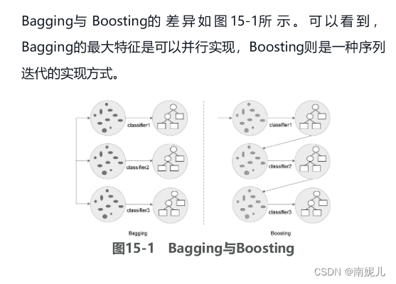
Bagging:另一种集成学习框架
Bagging是区别于Boosting的一种集成学习框架,通过对数据集自身采样来获取不同子集,并且对每个子集训练基分类器来进行模型集成。Bagging是一种并行化的集成学习方法。随机森林是Bagging学习框架的一个代表,通过样本和特征的两个随机性来构造基分类器,由多棵决策树进而形成随机森林
sklearn 代码实现
# 导入相关模块
from sklearn.datasets import make_classification
from sklearn.model_selection import train_test_split
import numpy as np
from sklearn.metrics import accuracy_score
# 生成模拟二分类数据集
X, y = make_classification(n_samples=1000,n_features=20,
                           n_redundant=0, n_informative=2,random_state=1,
                           n_clusters_per_class=1)
rng = np.random.RandomState(2)
X += 2 * rng.uniform(size=X.shape)
# 划分数据集
X_train, X_test, y_train, y_test = train_test_split(X, y, test_size=0.3)

# 导入随机森林分类器
from sklearn.ensemble import RandomForestClassifier
# 创建随机森林分类器实例
clf = RandomForestClassifier(max_depth=3, random_state=0)
# 模型拟合
clf.fit(X_train, y_train)
# 预测
y_pred = clf.predict(X_test)
acc = accuracy_score(y_test, y_pred)
# 输出分类准确率
print ("Accuracy of sklearn Random Forest:", acc)
集成学习:对比与调参
三大Boosting算法对比
XGBoost、LightGBM和CatBoost都是目前经典的SOTA(state of the art)Boosting算法,都可以归入梯度提升决策树算法系列。这三个模型都是以决策树为支撑的集成学习框架
第一,模型树的构造方式有所不同,XGBoost使用按层生长(level-wise)的决策树构建策略,LightGBM则使用按叶子生长(leaf-wise)的构建策略,而CatBoost使用对称树结构,其决策树都是完全二叉树。第二,对于类别特征的处理有较大区别,XGBoost本身不具备自动处理类别特征的能力,对于数据中的类别特征,需要我们手动处理变换成数值后才能输入到模型中;LightGBM中则需要指定类别特征名称,算法会自动对其进行处理;CatBoost以处理类别特征而闻名,通过目标变量统计等特征编码方式也能实现高效处理类别特征。
常用的超参数调优方法
机器学习模型中有大量参数需要事先人为设定,比如神经网络训练的batch-size、XGBoost等集成学习模型的树相关参数,我们将这类不是经过模型训练得到的参数叫作超参数(hyperparameter)。人为调整超参数的过程就是我们熟知的调参。机器学习中常用的调参方法包括网格搜索法(grid search)、随机搜索法(random search)和贝叶斯优化(bayesian optimization)
网格搜索法
网格搜索是一种常用的超参数调优方法,常用于优化三个或者更少数量的超参数,本质上是一种穷举法。对于每个超参数,使用者选择一个较小的有限集去探索,然后这些超参数笛卡儿乘积得到若干组超参数。网格搜索使用每组超参数训练模型,挑选验证集误差最小的超参数作为最优超参数。

### 基于XGBoost的GridSearch搜索范例
# 导入GridSearch模块
from sklearn.model_selection import GridSearchCV
# 创建xgb分类模型实例
model = xgb.XGBClassifier()
# 待搜索的参数列表空间
param_lst = {"max_depth": [3,5,7],
             "min_child_weight" : [1,3,6],
             "n_estimators": [100,200,300],
             "learning_rate": [0.01, 0.05, 0.1]
            }
# 创建网格搜索对象
grid_search = GridSearchCV(model, param_grid=param_lst, cv=3, verbose=10, n_jobs=-1)
# 基于flights数据集执行搜索
grid_search.fit(X_train, y_train)
# 输出搜索结果
print(grid_search.best_estimator_)
随机搜索
随机搜索,顾名思义,即在指定超参数范围内或者分布上随机搜寻最优超参数。相较于网格搜索方法,给定超参数分布,并不是所有超参数都会进行尝试,而是会从给定分布中抽样固定数量的参数,实际仅对这些抽样到的超参数进行实验。相较于网格搜索,随机搜索有时候会更高效
### 基于XGBoost的RandomizedSearch搜索范例
# 导入RandomizedSearchCV方法
from sklearn.model_selection import RandomizedSearchCV
# 创建xgb分类模型实例
model = xgb.XGBClassifier()
# 待搜索的参数列表空间
param_lst = {'max_depth': [3,5,7],
             'min_child_weight': [1,3,6],
             'n_estimators': [100,200,300],
             'learning_rate': [0.01, 0.05, 0.1]
            }
# 创建网格搜索
random_search = RandomizedSearchCV(model, param_lst, random_state=0)
# 基于flights数据集执行搜索
random_search.fit(X_train, y_train)
# 输出搜索结果
print(random_search.best_params_)
贝叶斯调参
贝叶斯优化是一种基于高斯过程(Gaussian process)和贝叶斯定理的参数优化方法,近年来广泛用于机器学习模型的超参数调优
### 基于XGBoost的BayesianOptimization搜索范例
# 导入xgb模块
import xgboost as xgb
# 导入贝叶斯优化模块
from bayes_opt import BayesianOptimization
# 定义目标优化函数
def xgb_evaluate(min_child_weight,
                 colsample_bytree,
                 max_depth,
                 subsample,
                 gamma,
                 alpha):
    # 指定要优化的超参数
    params['min_child_weight'] = int(min_child_weight)
    params['cosample_bytree'] = max(min(colsample_bytree, 1), 0)
    params['max_depth'] = int(max_depth)
    params['subsample'] = max(min(subsample, 1), 0)
    params['gamma'] = max(gamma, 0)
    params['alpha'] = max(alpha, 0)
    # 定义xgb交叉验证结果
    cv_result = xgb.cv(params, dtrain,
                       num_boost_round=num_rounds, nfold=5,
                       seed=random_state,
                       callbacks=[xgb.callback.early_stop(50)])
    return cv_result['test-auc-mean'].values[-1]
# 定义相关参数
num_rounds = 3000
random_state = 2021
num_iter = 25
init_points = 5
params = {
    'eta': 0.1,
    'silent': 1,
    'eval_metric': 'auc',
    'verbose_eval': True,
    'seed': random_state
}
# 创建贝叶斯优化实例
# 并设定参数搜索范围
xgbBO = BayesianOptimization(xgb_evaluate,
                             {'min_child_weight': (1, 20),
                              'colsample_bytree': (0.1, 1),
                              'max_depth': (5, 15),
                              'subsample': (0.5, 1),
                              'gamma': (0, 10),
                              'alpha': (0, 10),
                             })
# 执行调优过程
xgbBO.maximize(init_points=init_points, n_iter=num_iter)


 2018
2018


 被折叠的 条评论
为什么被折叠?
被折叠的 条评论
为什么被折叠?
 到【灌水乐园】发言


