Matplotlib画图

一、 Matplotlib画图

参考网址：https://mp.weixin.qq.com/s/p9cBY2C3vPbC1dR1n-jtrw

1.1、散点图

import numpy as np
import pandas as pd
import matplotlib as mpl
import matplotlib.pyplot as plt
import seaborn as sns
import warnings
warnings.filterwarnings(action='once')
pd.set_option('display.max_columns', 50)

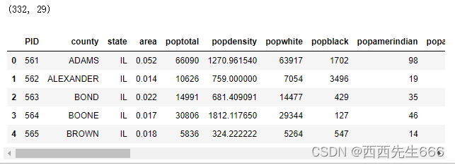
midwest = pd.read_csv("https://raw.githubusercontent.com/selva86/datasets/master/midwest_filter.csv")
print(midwest.shape)
midwest.head()

categories=np.unique(midwest.category)
print(len(categories))
colors=[plt.cm.tab10(i/float(len(categories))) for i in range(len(categories))]
colors
"""
14
[(0.12156862745098039, 0.4666666666666667, 0.7058823529411765, 1.0),
 (0.12156862745098039, 0.4666666666666667, 0.7058823529411765, 1.0),
 (1.0, 0.4980392156862745, 0.054901960784313725, 1.0),
 (0.17254901960784313, 0.6274509803921569, 0.17254901960784313, 1.0),
 (0.17254901960784313, 0.6274509803921569, 0.17254901960784313, 1.0),
 (0.8392156862745098, 0.15294117647058825, 0.1568627450980392, 1.0),
 (0.5803921568627451, 0.403921568627451, 0.7411764705882353, 1.0),
 (0.5490196078431373, 0.33725490196078434, 0.29411764705882354, 1.0),
 (0.5490196078431373, 0.33725490196078434, 0.29411764705882354, 1.0),
 (0.8901960784313725, 0.4666666666666667, 0.7607843137254902, 1.0),
 (0.4980392156862745, 0.4980392156862745, 0.4980392156862745, 1.0),
 (0.4980392156862745, 0.4980392156862745, 0.4980392156862745, 1.0),
 (0.7372549019607844, 0.7411764705882353, 0.13333333333333333, 1.0),
 (0.09019607843137255, 0.7450980392156863, 0.8117647058823529, 1.0)]
"""

plt.figure(figsize=(16,10),dpi=80,facecolor='w',edgecolor='k')#facecolor绘图区域的背景颜色,edgecolor绘图区域边界颜色
for i,category in enumerate(categories):
    plt.scatter('area','poptotal',
                data=midwest.loc[midwest.category==category,:],
                s=20,
                c=colors[i],
                label=str(category))
plt.gca().set(xlim=(0.0,0.1), #使用Plt.gca()获得当前子图(Get current Axes)
              ylim=(0,90000),
              xlabel='Area',
              ylabel='Population')
plt.xticks(fontsize=12); plt.yticks(fontsize=12)
plt.title("Scatterplot of Midwest Area vs Population", fontsize=22)
plt.legend(fontsize=12,loc='best')    
plt.show() 

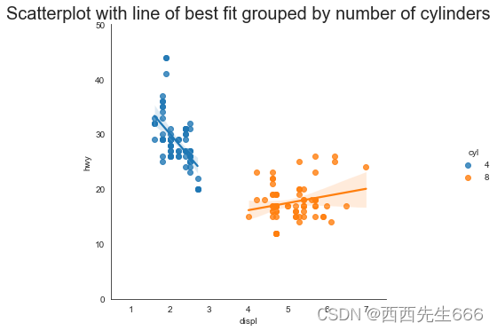
1.2、带线性回归最佳拟合线的散点图

df = pd.read_csv("https://raw.githubusercontent.com/selva86/datasets/master/mpg_ggplot2.csv")
df_select = df.loc[df.cyl.isin([4,8]), :]

# Plot
sns.set_style("white")
gridobj = sns.lmplot(x="displ", y="hwy", hue="cyl", data=df_select)

# Decorations
gridobj.set(xlim=(0.5, 7.5), ylim=(0, 50))
plt.title("Scatterplot with line of best fit grouped by number of cylinders", fontsize=20)

df = pd.read_csv("https://raw.githubusercontent.com/selva86/datasets/master/mpg_ggplot2.csv")
df_select = df.loc[df.cyl.isin([4,8]), :]

# Each line in its own column
sns.set_style("white")
gridobj = sns.lmplot(x="displ", y="hwy", 
                     data=df_select,
                     col="cyl")
# Decorations
gridobj.set(xlim=(0.5, 7.5), ylim=(0, 50))
plt.show()

参考网址：https://baijiahao.baidu.com/s?id=1704589568200942801&wfr=spider&for=pc

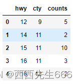
1.3、计数图

df = pd.read_csv("https://raw.githubusercontent.com/selva86/datasets/master/mpg_ggplot2.csv")
df_counts = df.groupby(['hwy', 'cty']).size().reset_index(name='counts')
df_counts.head()

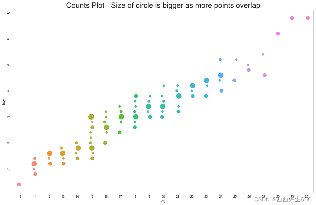
fig, ax = plt.subplots(figsize=(16,10), dpi= 80)    
sns.stripplot(df_counts.cty, df_counts.hwy, sizes=df_counts.counts*25, ax=ax) #stripplot散点图

# Decorations
plt.title('Counts Plot - Size of circle is bigger as more points overlap', fontsize=22)
plt.show()

1.4、边缘直方图

df = pd.read_csv("https://raw.githubusercontent.com/selva86/datasets/master/mpg_ggplot2.csv")

# Create Fig and gridspec
fig = plt.figure(figsize=(16, 10), dpi= 80)
grid = plt.GridSpec(4, 4, hspace=0.5, wspace=0.2)

# Define the axes
ax_main = fig.add_subplot(grid[:-1, :-1])
ax_right = fig.add_subplot(grid[:-1, -1], xticklabels=[], yticklabels=[])
ax_bottom = fig.add_subplot(grid[-1, :-1], xticklabels=[], yticklabels=[])

# Scatterplot on main ax
ax_main.scatter('displ', 'hwy', s=df.cty*4, 
                c=df.manufacturer.astype('category').cat.codes, data=df)

# histogram on the right
ax_bottom.hist(df.displ, bins=40, orientation='vertical')
ax_bottom.invert_yaxis()

# histogram in the bottom
ax_right.hist(df.hwy, bins=40, orientation='horizontal')

# Decorations
ax_main.set(title='Scatterplot with Histograms displ vs hwy', 
            xlabel='displ', ylabel='hwy')
ax_main.title.set_fontsize(20)
ax_main.xaxis.label.set_fontsize(20)
ax_main.yaxis.label.set_fontsize(20)
plt.show()

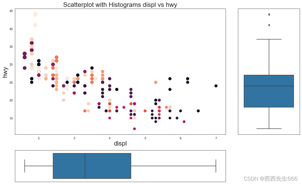
1.5、边缘箱型图

# Import Data
df = pd.read_csv("https://raw.githubusercontent.com/selva86/datasets/master/mpg_ggplot2.csv")

# Create Fig and gridspec
fig = plt.figure(figsize=(16, 10), dpi= 80)
grid = plt.GridSpec(4, 4, hspace=0.5, wspace=0.2)

# Define the axes
ax_main = fig.add_subplot(grid[:-1, :-1])
ax_right = fig.add_subplot(grid[:-1, -1], xticklabels=[], yticklabels=[])
ax_bottom = fig.add_subplot(grid[-1, :-1], xticklabels=[], yticklabels=[])

# Scatterplot on main ax
ax_main.scatter('displ', 'hwy', s=df.cty*5, 
                c=df.manufacturer.astype('category').cat.codes, data=df)

# Add a graph in each part
sns.boxplot(df.hwy, ax=ax_right, orient="v")
sns.boxplot(df.displ, ax=ax_bottom, orient="h")

# Remove x axis name for the boxplot
ax_bottom.set(xlabel='')
ax_right.set(ylabel='')

# Main Title, Xlabel and YLabel
ax_main.set(title='Scatterplot with Histograms displ vs hwy', 
            xlabel='displ', ylabel='hwy')

# Set font size of different components
ax_main.title.set_fontsize(20)
ax_main.xaxis.label.set_fontsize(20)
ax_main.yaxis.label.set_fontsize(20)
plt.show()

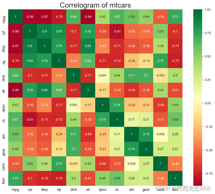
1.6、相关性图

# Import Dataset
df = pd.read_csv("https://github.com/selva86/datasets/raw/master/mtcars.csv")

# Plot
plt.figure(figsize=(12,10), dpi= 80)
sns.heatmap(df.corr(), 
            cmap='RdYlGn', 
            annot=True)

# Decorations
plt.title('Correlogram of mtcars', fontsize=22)
plt.xticks(fontsize=12)
plt.yticks(fontsize=12)
plt.show()