【机器学习】5.支持向量机（下）

1.SVM算法特性：

                                                        

    1.1 训练好的模型的算法复杂度是由支持向量的个数决定的，而不是由数据的维度决定的。所以SVM不太容易产生overfitting

    1.2 SVM训练出来的模型完全依赖于支持向量，即使训练集里面所有非支持向量的点都被去除，重复训练过程，结果仍然会得到完全一样的模型。

    1.3 一个SVM如果训练得出的支持向量个数比较小，SVM训练处的模型比较容易泛华。

2.线性不可分的情况

                                                            

    2.1 数据集在空间中对应的向量不可被一个超平面区分开

    2.2 两个步骤来解决：

        2.2.1 利用一个非线性的映射把原数据集中的向量点转换到一个更高维度的空间中

        2.2.2 在这个高维度的空间中找一个线性的超平面来根据线性可分的情况处理

                       

                    

2.3如何利用非线性映射把原始数据转换到高维中？

    2.3.1 例子：

        3维输入向量：

                                                                            

        转换到6维Z空间中：

                                                    

                                                    

        新的决策超平面：

                                                                            

    其中W和Z是向量，这个超平面的线性的，解出W和b之后，并且带入回原方程：

                                                    

    2.3.2问题的关键在于：

                                    (1)如何选择合理的非线性转换把数据转到高维度中

                                    (2)如何解决计算内积时算法复杂度非常高的问题

    2.3.3 使用核方法

3.核方法

    3.1 动机

        在线性SVM中转换为最优化问题时求解的公式计算都是以内积的形式出现的

                                                                        

        其中，是把训练集中的向量点转换到高维的非线性映射函数，因为内积的算法复杂度非常大，所以我们利用核函数来取代计算非线性映射函数的内积。

    3.2 以下核函数和非线性映射函数的内积等同

                                                                    

    3.3 常用的核函数

        h度多项式核函数

                                                                    

        高斯径向基核函数

                                                                    

        S型核函数

                                                                    

        选择使用哪个kernel主要根据先验知识，比如图像分类，通常使用RBF，文字不使用RBF，尝试不同的kernel，根据结果准确度而定。

    3.4 核函数举例

        假设定义两个向量：x=（x1,x2,x3）;y=(y1,y2,y3)

        定义方程：f(x)=(x1x1,x1x2,x1x3,x2x1,x2x2,x2x3,x3x1,x3x2,x3x3)

        K(x,y)=(<x,y>)^2

        假设x=（1,2,3）；y=(4,5,6)

        f(x)=(1,2,3,2,4,6,3,6,9)

        f(y)=(16,20,24,20,25,36,24,30,36)

        <f(x),f(y)>=16+40+72+40+100+180+72+180+324=1024

        K(x,y)=(4+10+18)^2=32^2=1024

        同样的结果，使用kernel方法计算容易得多

4. SVM扩展可解决多个类别分类问题

        对于每个类，有一个当前类和其他类的二类分类器。比如分10类，最开始设置一个分类器分第1类和第2到10类，然后分第2类和第3到10类，以此类推。

5.代码实例，用svm进行人脸识别

# -*- coding: utf-8 -*-

from __future__ import print_function

from time import time                       #在某些步骤计时
import logging                               #为了打印一些程序进展的信息
import matplotlib.pyplot as plt

from sklearn.cross_validation import train_test_split       #
from sklearn.datasets import fetch_lfw_people
from sklearn.grid_search import GridSearchCV
from sklearn.metrics import  classification_report
from sklearn.metrics import confusion_matrix
from sklearn.decomposition import RandomizedPCA
from sklearn.svm import SVC

logging.basicConfig(level=logging.INFO,format='%(asctime)s %(message)s')   #通过basicConfig把一些程序进展中的信息打印出来

lfw_people=fetch_lfw_people(min_faces_per_person=70,resize=0.4)   #下载LFW数据集

n_samples,h,w=lfw_people.images.shape           #返回数据集实例个数，参数

X=lfw_people.data          #特征向量的矩阵  每一行是一个实例，每一列是一个特征值ֵ
n_features=X.shape[1]       #每个人特征值个数

y=lfw_people.target         #目标分类的标记
target_names=lfw_people.target_names        #返回类别里的名字
n_classes=target_names.shape[0]    #返回数据集中人的个数

print('total dataset size:')
print('n_samples:%d'% n_samples)
print('n_features:%d'% n_features)
print('n_classes:%d'% n_classes)

X_train,X_test,y_train,y_test=train_test_split(
    X,y,test_size=0.25)                     #把数据集分成训练集和测试集矩阵

##将特征值降维，提高预测准确性
n_components=150        #组成元素的数量
print('Extracting the top %d eigenfaces from %d faces'
      %(n_components,X_train.shape[0]))
t0=time()   #起始一个初始时间
pca=RandomizedPCA(n_components=n_components,whiten=True).fit(X_train)   #随机降维训练集里的特征向量
print("done in %0.3fs"%(time()-t0))

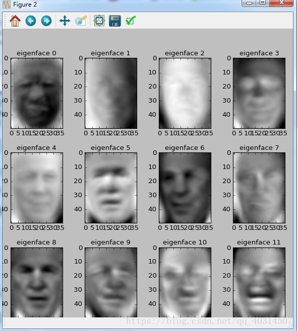
eigenfaces=pca.components_.reshape((n_components,h,w))     #在人脸上提取特征值
t0=time()
x_train_pca=pca.transform(X_train)      #把x_train转换成更低维的矩阵
x_test_pca=pca.transform(X_test)        #把y_train转换成更低维的矩阵
print("done in %0.3fs"%(time()-t0))
####

##对提取出的特征值进行分类
print("Fitting the classifier to training set")
to=time()
param_grid={'C':[1e3,5e3,1e4,5e4,1e5],
            'gamma':[0.0001,0.0005,0.001,0.005,0.01,0.1],}      #调用不同参数，看哪个效果好
clf=GridSearchCV(SVC(kernel='rbf',class_weight='auto'),param_grid)
clf=clf.fit(x_train_pca,y_train)
print("done in %0.3fs"%(time()-t0))
print(clf.best_estimator_)          
###

##评估
print("Predicting people's names on the test set ")
t0=time()
y_pred=clf.predict(x_test_pca)
print("done in %0.3fs"%(time()-t0))

print(classification_report(y_test,y_pred,target_names=target_names))       #评判分类器预测能力
print(confusion_matrix(y_test, y_pred, labels=range(n_classes)))            #真实标记和预测标记差别
##

def plot_gallery(images,titles,h,w,n_row=3,n_col=4):
    """helper function to plot a gallery of portraits"""
    plt.figure(figsize=(1.8*n_col,2.4*n_row))
    plt.subplots_adjust(bottom=0,left=.01,right=.99,top=.90,hspace=.35)
    for i in range(n_row*n_col):
        plt.subplot(n_row,n_col,i+1)
        plt.imshow(images[i].reshape((h,w)),cmap=plt.cm.gray)
        plt.title(titles[i],size=12)
        plt.xticks()
        plt.yticks()
    
      
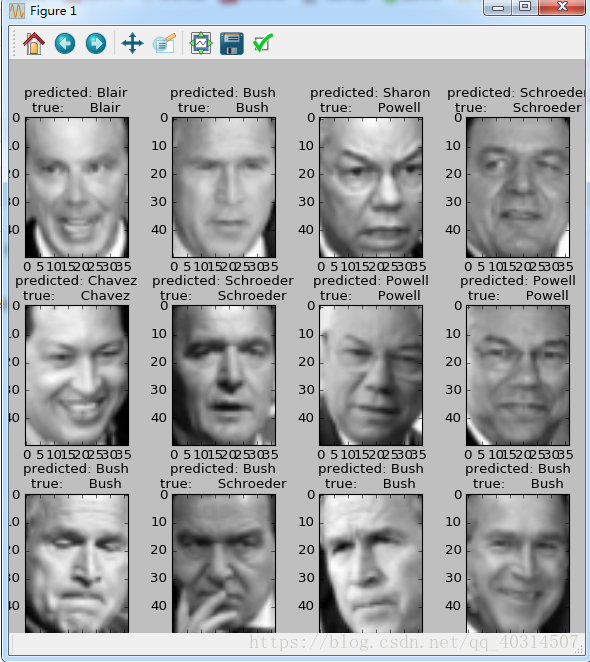
def title(y_pred,y_test,target_names,i):
    pred_name = target_names[y_pred[i]].rsplit(' ', 1)[-1]
    true_name=target_names[y_test[i]].rsplit(' ',1)[-1]
    
    return 'predicted: %s\ntrue:      %s' % (pred_name, true_name)
prediction_titles=[title(y_pred,y_test,target_names,i)
                   for i in range(y_pred.shape[0])]
plot_gallery(X_test, prediction_titles, h, w)
eigenface_titles = ["eigenface %d" % i for i in range(eigenfaces.shape[0])]
plot_gallery(eigenfaces, eigenface_titles, h, w)
plt.show()