


文章目录
ZFnet论文链接:https://arxiv.org/pdf/1311.2901.pdf
摘要:大型卷积网络模型最近在 ImageNet数据集上展示了令人印象深刻的分类性能(Krizhevsky 等)。但是它们为什么表现如此出色?或者如何改进它们?到现在为止还没有一个清晰的理解。在本文中我们解决了这两个问题。我们引入了一种新颖的可视化技术,可以深入了解***中间特征层的功能***和***分类器的操作***。 这些可视化方法使我们能够***找到优于 AlexNet的模型架构***。 在 ImageNet 分类基准上,我们还进行了***消融研究,以发现不同模型层的性能贡献***。 我们展示了我们的 ImageNet 模型很好地推广到其他数据集:当重新训练 softmax 分类器时,它取得了 Caltech-101 和 Caltech-256 数据集上当前最先进的结果。
一、介绍
1、深度学习为什么会有如此大的突破呢?
①大规模结构化数据集;②GPU发展快;③Dropout等模型正则化方法
2、揭示了convnet的内部操作以及复杂模型的行为。本文介绍了:
①一种揭示网络中间层哪些输入特征能激活特征图的可视化技巧(多层反卷积网络),deconvnet将特征激活部分投影回输入的像素空间;
②可以在训练期间观察特征演化并诊断模型中的潜在问题;
③遮挡输入图像的部分来对分类器的输出进行敏感性分析,揭示场景中哪些部分对分类比较重要。
3、相关工作
可视化特征,本文所用方法提供了一个参数不变性视图,显示了训练集上的哪些模式能激活特定的特征图。本文可视化方法既有输入图像裁剪的方法也有从后向前投影的方法(deconvnet)揭示网络结构中每一个小块能激活哪个特定的特征图
二、方法(有监督学习)
使用了标准的全卷积网络,这些模型将一个三通道的2D图像映射为C个类别的向量。每一层包含①来自上一个卷积层的输出结果以及可学习的卷积核集合②ReLU③局部近邻的最大池化层(可选)④对比度归一化层(可选)⑤网络最顶部的几层是FC层⑥最后一层是softmax层。
训练方法:多分类交叉熵损失函数,反向传播和梯度下降训练网络中的一些参数(卷积核权重以及全连接权重),通过随机梯度下降更新每一个参数。
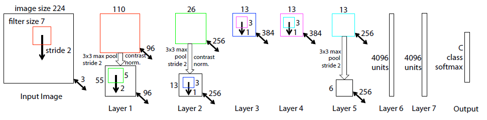
结构为本文的8层卷积网络模型。
图像裁剪为224×224大小作为网络的输入,先与96个不同的第一层过滤器进行卷积运算(kernel_size=7, 在框x和y上的stride=2)。然后进行如下步骤:①通过整流线性激活函数;②最大池化(kernel_size=3, stride=2);③跨特征图对比度归一化操作得到96个不同的55×55大小的特征图。第2、3、4、5层重复类似操作。
最后两层为FC层,将顶部卷积层的特征作为向量形式的输入(6×6×256=9016维)。
最后一层为C通道softmax层,其中C为类别数。
1、反卷积网络(可视化)
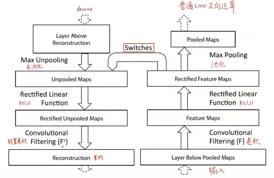
方法概述:将中间特征层的激活映射到输入图像的像素空间,就能显示输入中的哪些模式特征能够导致某一个中间层的特征图被激活。DeconvNet其实就是卷积操作的反操作,即转置卷积、反激活、反池化,将特征映射到像素(卷积是将像素映射到特征形成特征图)。
反卷积网络实现步骤:
①输入图像进入到卷积层中进行正向计算得到特征,并挑出我们想要可视化的特征图,除了所挑选的这张特征图之外的所有特征图我们都将之设置为0,将挑选的特征图传入到deconvnet中;
②依次进行反池化、反激活(ReLU)、转置卷积操作;
③在到达输入像素空间之前重复步骤②。
1.1、反池化(上采样)
下采样与上采样的定义
缩小图像(或称为下采样(subsampled)或降采样(downsampled))的主要目的有两个:1、使得图像符合显示区域的大小;2、生成对应图像的缩略图。
放大图像(或称为上采样(upsampling)或图像插值(interpolating))的主要目的是放大原图像,从而可以显示在更高分辨率的显示设备上。
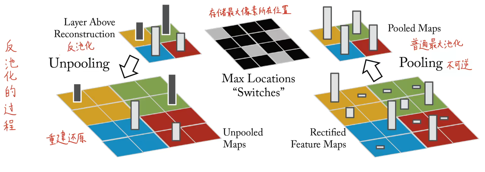
最大池化不可逆转,因为池化操作(下采样)是将大图转变为小图丢失了很多空间信息,从小图变为大图几乎是不可能实现的。但是文章使用了switch操作(池化时记录下最大值像素的位置,反池化时就将按照该位置派遣此最大值即可),不可避免的是仍然会丢失其他像素的信息,但是不会影响大局。
1.2、反激活
卷积网络使用ReLU非线性激活函数,它修正了特征图使得特征图的值始终为正值,为了在每一层(特征图也需保证均为正值)都得到有效的特征重建,依旧使用ReLU函数来进行重建。
1.3、转置(反)卷积
使用转置后的卷积核(正向卷积使用过的学习后的卷积核),即将卷积核水平或垂直翻转。但是该卷积核是应用在修正后的特征图上而不是下层的输出上。反卷积中没有学习任何参数,是完全无监督的。
从更高层使用由convnet中的最大池化产生的switch操作设置向下层投影,虽然池化时会丢失一部分信息,但重构得到的图和原始输入图依旧很像,亮暗轮廓体现出特定特征图反应的特征。需要注意的是:投影回原始像素空间的图像不是原始数据集中的样本,中间过程并没有生成新的图像。
三、训练细节
1、数据集:使用ImageNet的数据集。
2、网络训练模式:与AlexNet不同之处在于ZFnet使用密集连接方式(使用一个GPU)
3、数据预处理:每张图片都将最短维resize到256,裁剪中心的256×256区域,使用去均值化处理,然后再这个基础上取出中间+四角的224*224的图像再取水平翻转后的图像(共10张不同的)
4、优化器:小批次尺寸为128的随机梯度下降(SGD)优化器更新参数,学习率为0.01,动量为0.9.验证集错误率停止减小,那么就在训练时手动减小学习率。
5、防止过拟合:Dropout(用在FC层,即第6、7层)率为0.5。
6、初始化权重:所有权重都初始化为0.01且偏置为0。
7、训练期间第一层卷积核的可视化揭示了其中的一些卷积核占据主导地位,为解决此问题,将卷积层中RMS值超过0.1的固定半径的每个卷积核重新归一化到这个固定半径,这一点对第一层至关重要,输入图像范围大致在[-128, 128]。
8、训练了70个epoch停止,实施方式同AlexNet.
四、卷积网络可视化

第一层(底层网络)提取的是底层特征,比如边缘、转角、颜色等等特征,第一层卷积层不需要deconvnet,直接提取即可。
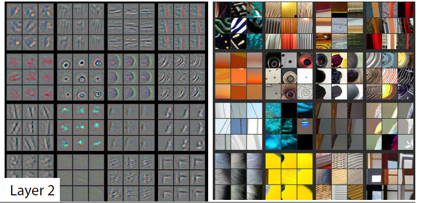
第二层:左图为输入中间层的特征图用deconvnet重构回原输入像素空间后得到的图,右图为能够使第二层某个特征图最大激活的前9个patch,每个patch都来自验证集。左边的图和右边的图是一一对应的,只不过左边的图是第二层卷积核得到的特征图通过deconvnet之后映射回原像素空间可视化得到的图像。
特征图体现了输入图像中符合卷积核定义特征的一些特征,可视化出的特征图间接反映了卷积核到底提取到了一些什么样的特征,如第一大行第二大列提取出的特征为条纹特征。

第三层deconv重构得到的图开始出现了形状信息。后面的层的特征越来越高级,随着网络越来越深,提取的特征越具有特征不变性(关注语义信息),即能够从不同的物体中提取到相同的特征(语义信息)。
怎么得到左图的呢?
答:从原始数据中找出能够使得某个特征图在训练的某个批次激活最大的原图,然后把原图传入到网络中求出该特征图的值,再将特征图用deconvnet方法重构回原始像素输入空间,可视化原始像素空间就能够得到左图中对应于这个特征图的图片。
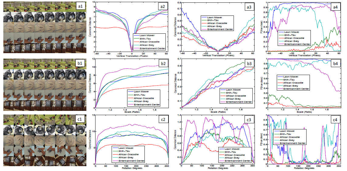
特征不变性:若对图片进行平移、旋转、缩放,在底层网络中对提取的特征图会造成很大的影响;在中高层网络中对提取的特征图会造成准线性的影响,不会非常大,此时网络对旋转还是比较敏感的(除非旋转到了对称位置)。
4.1、模型改进
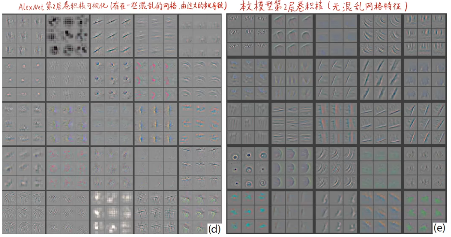
问题:AlexNet中第一层卷积核有一些特别高或者特别低的高频信息,这些卷积核都是无效卷积核;第二层卷积核可视化显示了由第一层步幅为4的卷积导致的混叠特征。
改进方法:(i) 将第一个卷积核大小由11×11改变为7×7; (ii) 将第一、二层卷积步幅由4变为2。
改变结果:(i) 新模型在第一、二层特征中保留了更多的信息; (ii)提高了分类性能。

4.2、局部遮挡敏感性分析
问题:网络是用关键局部信息进行分类还是用周围元素进行分类呢?
答案:网络是对关键部位感兴趣,若关键部位被遮挡,那么网络准确率会降低。


4.3、图像的局部相关性分析
深度学习区别于现存的识别方法是深度学习模型没有显示地定义图像中各部分的关系。
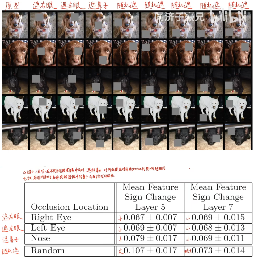
从第一行到第四行数据的对比说明了狗的眼睛、鼻子是被隐式地定义在了模型中;第二列与第三列对比再次说明了网络层数越深特征不变性这个性质越强,遮挡对特征图的计算影响越小。
五、实验
5.1、ImageNet 2012
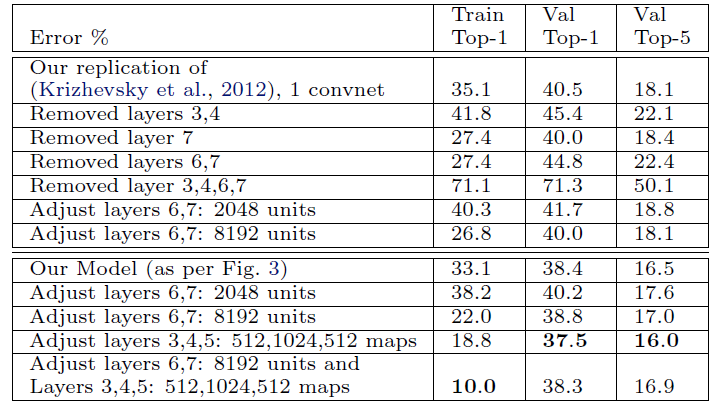
1:仅去掉网络中第六、七层(FC层),错误率会稍微减少。对之后网络改进的影响有:将FC层变为GAP层,可以提升网络性能的同时减少参数量防止过拟合。
2、仅去掉两个中间的卷积层,对网络性能影响不大。
3、将上述两个实验中的层都去掉,网络性能变差,得出结论:网络深度对性能影响是正向的。
4、改变FC层中神经元的个数,对网络性能影响不大。
5、增加卷积层中卷积核个数,使得网络性能变好,但是这会扩大FC层中的参数量最终导致过拟合。
总结
本论文提出了一种可视化神经网络中间层的方法(deconvnet),打开了CNN这个黑箱子,让我们知道了每个神经元是在提取什么特征,利用这些可视化技巧,得到中间提取的特征的deconvnet的图像,我们可以更好地改进网络。对AlexNet的第一、二层卷积层稍微进行了改动。
1、deconvnet步骤为:反池化、反激活(ReLU)、反卷积
1、底层网络体现特征:边缘、颜色; 中层网络体现特征:形状; 高层网络体现特征:物体
2、AlexNet中第一层卷积核大小由11×11→7×7,第一、二层卷积核步长改变为2
ZFNet代码实现(pytorch)
import torch.nn as nn
import torch
class ZFNet(nn.Module):
    def __init__(self, num_classes=1000, init_weights=False):
        super(ZFNet, self).__init__()
        self.features = nn.Sequential(
            nn.Conv2d(3, 96, kernel_size=7, stride=2, padding=0),   # [3, 227, 227] → [96, 111, 111]
            nn.ReLU(inplace=True),
            nn.MaxPool2d(kernel_size=3, stride=2, padding=0),        # [96, 111, 111] → [96, 55, 55]
            nn.Conv2d(96, 256, kernel_size=5, stride=2, padding=1),  # [96, 55, 55] → [256, 27, 27]
            nn.ReLU(inplace=True),
            nn.MaxPool2d(kernel_size=3, stride=2),                   # [256, 27, 27] → [256, 13, 13]
            nn.Conv2d(256, 384, kernel_size=3, stride=1, padding=1), # [256, 13, 13] → [384, 13, 13]
            nn.ReLU(inplace=True),
            nn.Conv2d(384, 384, kernel_size=3, stride=1, padding=1), # [384, 13, 13] → [384, 13, 13]
            nn.ReLU(inplace=True),
            nn.Conv2d(384, 256, kernel_size=3, stride=1, padding=1), # [384, 13, 13] → [256, 13, 13]
            nn.ReLU(inplace=True),
            nn.MaxPool2d(kernel_size=3, stride=2, padding=0),        # [256, 13, 13] → [256, 6, 6]
        )
        self.classifier = nn.Sequential(
            nn.Dropout(p=0.5),
            nn.Flatten(),
            nn.Linear(256 * 6 * 6, 2048),
            nn.ReLU(inplace=True),
            nn.Dropout(p=0.5),
            nn.Linear(2048, 2048),
            nn.ReLU(inplace=True),
            nn.Linear(2048, num_classes),
        )
        if init_weights:
            self._initialize_weights()

    def forward(self, x):
        x = self.features(x)
        x = torch.flatten(x, start_dim=1)
        x = self.classifier(x)
        return x

    def _initialize_weights(self):
        for m in self.modules():
            if isinstance(m, nn.Conv2d):
                nn.init.kaiming_normal_(m.weight, mode='fan_out', nonlinearity='relu')
                if m.bias is not None:
                    nn.init.constant_(m.bias, 0)
            elif isinstance(m, nn.Linear):
                nn.init.normal_(m.weight, 0, 0.01)
                nn.init.constant_(m.bias, 0)


# 使用torch.summary()函数得到网络各层的输出结果并打印
from torchsummary import summary
# 需要使用device来指定网络在GPU还是CPU运行
device = torch.device('cuda' if torch.cuda.is_available() else 'cpu')
# 建立神经网络模型,这里直接导入已有模型
model = ZFNet().to(device)
# 使用summary,注意输入维度的顺序
summary(model, input_size=(3, 227, 227))
top_layer = model.layers[0]
plt.imshow(top_layer.get_weights()[0][:, :, :, 0].squeeze(), cmap='gray')
可视化网络中间层特征图(pytorch)
方法一:
import cv2
import numpy as np
import torch
from torch.autograd import Variable
from torchvision import models
from torchsummary import summary

def preprocess_image(cv2im, resize_im=True):
    """
        Processes image for CNNs
    Args:
        PIL_img (PIL_img): Image to process
        resize_im (bool): Resize to 224 or not
    returns:
        im_as_var (Pytorch variable): Variable that contains processed float tensor
    """
    # mean and std list for channels (Imagenet)
    mean = [0.485, 0.456, 0.406]
    std = [0.229, 0.224, 0.225]
    # Resize image
    if resize_im:
        cv2im = cv2.resize(cv2im, (224, 224))
    im_as_arr = np.float32(cv2im)
    im_as_arr = np.ascontiguousarray(im_as_arr[..., ::-1])
    im_as_arr = im_as_arr.transpose(2, 0, 1)  # Convert array to D,W,H
    # Normalize the channels
    for channel, _ in enumerate(im_as_arr):
        im_as_arr[channel] /= 255
        im_as_arr[channel] -= mean[channel]
        im_as_arr[channel] /= std[channel]
    # Convert to float tensor
    im_as_ten = torch.from_numpy(im_as_arr).float()
    # Add one more channel to the beginning. Tensor shape = 1,3,224,224
    im_as_ten.unsqueeze_(0)
    # Convert to Pytorch variable
    im_as_var = Variable(im_as_ten, requires_grad=True)
    return im_as_var


class FeatureVisualization():
    def __init__(self,img_path,selected_layer):
        self.img_path=img_path
        self.selected_layer=selected_layer
        self.pretrained_model = models.vgg16(pretrained=True).features

    def process_image(self):
        img = cv2.imread(self.img_path)
        img = preprocess_image(img)
        return img

    def get_feature(self):
        # input = Variable(torch.randn(1, 3, 224, 224))
        input = self.process_image()
        print(input.shape)
        x = input
        for index, layer in enumerate(self.pretrained_model):
            x = layer(x)
            if (index == self.selected_layer):
                return x

    def get_single_feature(self):
        features=self.get_feature()
        print(features.shape)

        feature=features[:,0,:,:]
        print(feature.shape)

        feature=feature.view(feature.shape[1],feature.shape[2])
        print(feature.shape)

        return feature

    def save_feature_to_img(self):
        #to numpy
        feature=self.get_single_feature()
        feature=feature.data.numpy()

        #use sigmod to [0,1]
        feature= 1.0/(1+np.exp(-1*feature))

        # to [0,255]
        feature=np.round(feature*255)
        print(feature[0])

        cv2.imwrite('C:\\Users\\DavidLee\\Desktop\\img.jpg', feature)

if __name__=='__main__':
    # get class
    myClass=FeatureVisualization('C:\\Users\\DavidLee\\Desktop\\fish.jpeg', 9)  # 取网络中层数的索引值
    device = torch.device('cuda' if torch.cuda.is_available() else 'cpu')
    model = models.vgg16(pretrained=True).to(device)
    summary(model, input_size=(3, 224, 224))
    print (myClass.pretrained_model)
    myClass.save_feature_to_img()
使用模型为:VGG16预训练模型
初始图片为:

当网络索引数为5时,输出图像为:

当网络索引数为9时,输出图像为:

当网络索引数为9时,输出图像为:

总结:此方法虽然能求出各个层上特征图deconvnet后映射到原始图像空间的图片,但是显然没有达到本文的网络越深特征体现越鲜明的要求。
方法二:
import torch
from torchvision import models, transforms
from PIL import Image
import matplotlib.pyplot as plt
import numpy as np
import imageio
plt.rcParams['font.sans-serif'] = ['STSong']

model = models.alexnet(pretrained=True)
# 1.模型查看
print(model)     #可以看出网络一共有3层,两个Sequential()+avgpool
# 2. 导入数据
# 以RGB格式打开图像
# Pytorch DataLoader就是使用PIL所读取的图像格式
# 建议就用这种方法读取图像,当读入灰度图像时convert('')
def get_image_info(image_dir):
    image_info = Image.open(image_dir).convert('RGB')  # 是一幅图片
    # 数据预处理方法
    image_transform = transforms.Compose([
        transforms.Resize(256),
        transforms.CenterCrop(224),
        transforms.ToTensor(),
        transforms.Normalize([0.485, 0.456, 0.406], [0.229, 0.224, 0.225])
    ])
    image_info = image_transform(image_info)  # torch.Size([3, 224, 224])
    image_info = image_info.unsqueeze(0)  # torch.Size([1, 3, 224, 224])因为model的输入要求是4维,所以变成4维
    return image_info  # 变成tensor数据

# 2. 获取第k层的特征图
'''
args:
k:定义提取第几层的feature map
x:图片的tensor
model_layer:是一个Sequential()特征层
'''

def get_k_layer_feature_map(model_layer, k, x):
    with torch.no_grad():
        for index, layer in enumerate(model_layer):  # model的第一个Sequential()是有多层,所以遍历
            x = layer(x)  # torch.Size([1, 64, 55, 55])生成了64个通道
            if k == index:
                return x

#  可视化特征图
def show_feature_map(feature_map):  # feature_map=torch.Size([1, 64, 55, 55]),feature_map[0].shape=torch.Size([64, 55, 55])
    # feature_map[2].shape     out of bounds
    feature_map = feature_map.squeeze(0)  # 压缩成torch.Size([64, 55, 55])

    # 以下4行,通过双线性插值的方式改变保存图像的大小
    feature_map = feature_map.view(1, feature_map.shape[0], feature_map.shape[1], feature_map.shape[2])  # (1,64,55,55)
    upsample = torch.nn.UpsamplingBilinear2d(size=(256, 256))  # 这里进行调整大小
    feature_map = upsample(feature_map)
    feature_map = feature_map.view(feature_map.shape[1], feature_map.shape[2], feature_map.shape[3])

    feature_map_num = feature_map.shape[0]  # 返回通道数
    row_num = np.ceil(np.sqrt(feature_map_num))  # 8
    plt.figure()
    transfer = transforms.Compose([transforms.ToTensor(),
                                   transforms.ToPILImage()])
    for index in range(1, feature_map_num + 1):  # 通过遍历的方式,将64个通道的tensor拿出
        plt.subplot(row_num, row_num, index)
        plt.imshow(feature_map[index - 1], cmap='gray')  # feature_map[0].shape=torch.Size([55, 55])
        # 将上行代码替换成,可显示彩色 plt.imshow(transforms.ToPILImage()(feature_map[index - 1]))#feature_map[0].shape=torch.Size([55, 55])
        plt.axis('off')
        imageio.imwrite('feature_map_save//' + str(index) + ".png", feature_map[index - 1])
    plt.show()

if __name__ == '__main__':
    image_dir = r"horse.png"
    # 定义提取第几层的feature map
    k = 3
    image_info = get_image_info(image_dir)
    model = models.alexnet(pretrained=True)
    model_layer = list(model.children())
    model_layer = model_layer[0]  # 这里选择model的第一个Sequential()
    feature_map = get_k_layer_feature_map(model_layer, k, image_info)
    show_feature_map(feature_map)
使用模型为:AlexNet预训练模型
初始输入图片为:
提取第0层特征图deconvnet图像结果为: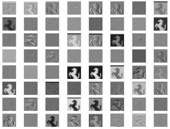
提取第3层特征图deconvnet图像结果为: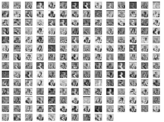
提取第7层特征图deconvnet图像结果为: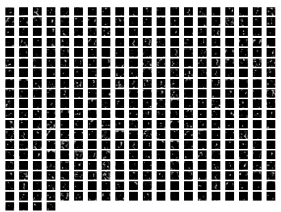
方法三:
# -*- coding: utf-8 -*-
import os
import shutil
import time
import torch
import torch.nn as nn
from torchvision import transforms
from torchvision import datasets
import torchvision.utils as vutil
from torch.utils.data import DataLoader
import torchsummary

DEVICE = torch.device("cuda" if torch.cuda.is_available() else "cpu")
EPOCH = 1
LR = 0.001
TRAIN_BATCH_SIZE = 64
TEST_BATCH_SIZE = 32
BASE_CHANNEL = 32
INPUT_CHANNEL = 1
INPUT_SIZE = 28
MODEL_FOLDER = './save_model'
IMAGE_FOLDER = './save_image'
INSTANCE_FOLDER = None


class AlexNet(nn.Module):
    def __init__(self, input_ch, num_classes, base_ch):
        super(AlexNet, self).__init__()

        self.num_classes = num_classes
        self.base_ch = base_ch
        self.feature_length = base_ch * 4

        self.conv1 = nn.Sequential(nn.Conv2d(input_ch, base_ch, kernel_size=3, padding=1),
                                   nn.ReLU(),
                                   nn.MaxPool2d(kernel_size=2, stride=1))

        self.conv2 = nn.Sequential(nn.Conv2d(base_ch, 2 * base_ch, kernel_size=3, padding=1),
                                   nn.ReLU(),
                                   nn.MaxPool2d(kernel_size=2, stride=1))

        self.conv3 = nn.Sequential(nn.Conv2d(base_ch * 2, 3 * base_ch, kernel_size=3, padding=1),
                                   nn.ReLU(),
                                   nn.MaxPool2d(kernel_size=2, stride=2))

        self.conv4 = nn.Sequential(nn.Conv2d(base_ch * 3, 4 * base_ch, kernel_size=3, padding=1),
                                   nn.ReLU(),
                                   nn.MaxPool2d(kernel_size=2, stride=2))

        self.conv5 = nn.Sequential(nn.Conv2d(base_ch * 4, self.feature_length, kernel_size=3, padding=1),
                                   nn.ReLU(),
                                   nn.AdaptiveAvgPool2d(output_size=(1, 1)))

        self.dense = nn.Sequential(nn.Linear(self.feature_length, 120),
                                   nn.ReLU(),
                                   nn.Linear(120, 84),
                                   nn.ReLU(),
                                   nn.Linear(84, 10))

    def forward(self, input):
        output = self.conv1(input)
        output = self.conv2(output)
        output = self.conv3(output)
        output = self.conv4(output)
        output = self.conv5(output)
        output = output.view(-1, self.feature_length)
        output = self.dense(output)
        return output

    def _initialize_weights(self):
        for m in self.modules():
            if isinstance(m, nn.Conv2d):
                nn.init.kaiming_normal_(m.weight, mode='fan_out', nonlinearity='relu')
                if m.bias is not None:
                    nn.init.constant_(m.bias, 0)
            elif isinstance(m, nn.Linear):
                nn.init.normal_(m.weight, 0, 0.01)
                nn.init.constant_(m.bias, 0)

def load_dataset():
    train_dataset = datasets.MNIST(root='./data',
                                   train=True,
                                   transform=transforms.ToTensor(),
                                   download=True)
    test_dataset = datasets.MNIST(root='./data',
                                  train=False,
                                  transform=transforms.ToTensor(),
                                  download=True)
    return train_dataset, test_dataset


def hook_func(module, input, output):
    """
    Hook function of register_forward_hook

    Parameters:
    -----------
    module: module of neural network
    input: input of module
    output: output of module
    """
    image_name = get_image_name_for_hook(module)
    data = output.clone().detach()
    print(data.size())
    data = data.permute(1, 0, 2, 3)
    # data = data.view(data.shape[0], data.shape[2], data.shape[3])
    vutil.save_image(data, image_name, pad_value=0.5)


def get_image_name_for_hook(module):
    """
    Generate image filename for hook function

    Parameters:
    -----------
    module: module of neural network
    """
    os.makedirs(INSTANCE_FOLDER, exist_ok=True)
    base_name = str(module).split('(')[0]
    index = 0
    image_name = '.'  # '.' is surely exist, to make first loop condition True
    while os.path.exists(image_name):
        index += 1
        image_name = os.path.join(INSTANCE_FOLDER, '%s_%d.png' % (base_name, index))
    return image_name


if __name__ == '__main__':
    time_beg = time.time()

    train_dataset, test_dataset = load_dataset()
    train_loader = DataLoader(dataset=train_dataset,
                              batch_size=TRAIN_BATCH_SIZE,
                              shuffle=True)
    test_loader = DataLoader(dataset=test_dataset,
                             batch_size=TEST_BATCH_SIZE,
                             shuffle=False)

    model = AlexNet(input_ch=1, num_classes=10, base_ch=BASE_CHANNEL).cuda()
    torchsummary.summary(model, input_size=(INPUT_CHANNEL, INPUT_SIZE, INPUT_SIZE))
    criterion = nn.CrossEntropyLoss()
    optimizer = torch.optim.Adam(model.parameters(), lr=LR)

    train_loss = []
    for ep in range(EPOCH):
        # ----------------- train -----------------
        model.train()
        time_beg_epoch = time.time()
        loss_recorder = []
        for data, classes in train_loader:
            data, classes = data.cuda(), classes.cuda()
            optimizer.zero_grad()
            output = model(data)
            loss = criterion(output, classes)
            loss.backward()
            optimizer.step()

            loss_recorder.append(loss.item())
            time_cost = time.time() - time_beg_epoch
            print('\rEpoch: %d, Loss: %0.4f, Time cost (s): %0.2f' % ((ep+1), loss_recorder[-1], time_cost), end='')

        # print train info after one epoch
        train_loss.append(loss_recorder)
        mean_loss_epoch = torch.mean(torch.Tensor(loss_recorder))
        time_cost_epoch = time.time() - time_beg_epoch
        print('\rEpoch: %d, Mean loss: %0.4f, Epoch time cost (s): %0.2f' % ((ep+1), mean_loss_epoch.item(), time_cost_epoch), end='')

        # save model
        os.makedirs(MODEL_FOLDER, exist_ok=True)
        if (ep + 1) % 5 == 0:
            model_filename = os.path.join(MODEL_FOLDER, 'epoch_%d.pth' % (ep + 1))
            torch.save(model.state_dict(), model_filename)

        # ----------------- test -----------------
        model.eval()
        correct = 0
        total = 0
        for data, classes in test_loader:
            data, classes = data.cuda(), classes.cuda()
            output = model(data)
            _, predicted = torch.max(output.data, 1)
            total += classes.size(0)
            correct += (predicted == classes).sum().item()
        print(', Test accuracy: %0.4f' % (correct / total))

    print('Total time cost: ', time.time() - time_beg)

    # ----------------- visualization -----------------
    # clear output folder
    if os.path.exists(IMAGE_FOLDER):
        shutil.rmtree(IMAGE_FOLDER)

    model.eval()
    modules_for_plot = (torch.nn.ReLU, torch.nn.Conv2d,
                        torch.nn.MaxPool2d, torch.nn.AdaptiveAvgPool2d)
    for name, module in model.named_modules():
        if isinstance(module, modules_for_plot):
            module.register_forward_hook(hook_func)

    test_loader = DataLoader(dataset=test_dataset,
                             batch_size=1,
                             shuffle=False)
    index = 1
    for data, classes in test_loader:
        INSTANCE_FOLDER = os.path.join(IMAGE_FOLDER, '%d-%d' % (index, classes.item()))
        data, classes = data.cuda(), classes.cuda()
        outputs = model(data)
        index += 1
        if index > 20:
            break
输入图片为MNIST手写数字识别图片集,所用模型为AlexNet
输出结果为:
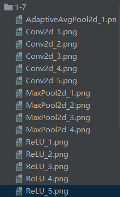
结果解释:文件夹名字1-7表示第一个图片索引以及第一个图片的类别
底下是各个层特征图deconvnet出来的图片,可以看出此方法与本文的方法最接近。
方法四:调用现成的包
from Evison import Display, show_network
from torchvision import models
from PIL import Image

network = models.alexnet(pretrained=True)
show_network(network)

visualized_layer = 'features.12'
display = Display(network, visualized_layer, img_size=(224, 224))
image = Image.open('fish.jpeg').resize((224, 224))
display.save(image, file='%s' % visualized_layer)
输入图像:
输出图像:
第七层灰度图: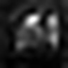
第七层热力图: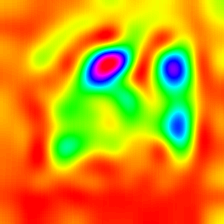
第七层CAM图: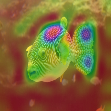
引用文章
[1] 下采样与上采样 - 小虾米的java梦 - 博客园 (cnblogs.com)
[2] 【精读AI论文】ZFNet深度学习图像分类算法(反卷积可视化可解释性分析)_哔哩哔哩_bilibili
[3] PyTorch | 提取神经网络中间层特征进行可视化 - 简书 (jianshu.com)
[4] pytorch实现特征图可视化,代码简洁,包教包会_Mr_DaYang的博客-CSDN博客_pytorch特征图可视化


 1306
1306


 被折叠的 条评论
为什么被折叠?
被折叠的 条评论
为什么被折叠?
 到【灌水乐园】发言


