电影推荐系统

电影推荐系统

常见的电影推荐系统算法有协同过滤和矩阵因子分解。而协同过滤算法有基于item和基于user两种不同的形式。
数据来自：
here.
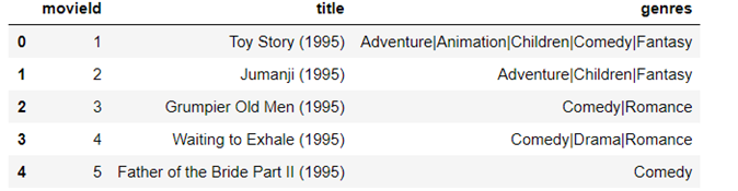
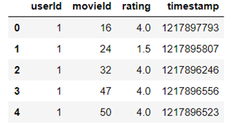
部分数据展示如下：movies.csv（shape:103293）和ratings.csv（shape:1053394）

进行简单的数据分析

Most Viewed Movies Visualization：we will explore the most viewed movies in our dataset. We will first count the number of views in a film and then organize them in a table that would group them in descending order.

we will visualize the distribution of the average ratings per user.

评分均值的mean = 3.66，std=0.456。
实现它们的代码如下：

import pandas as pd
import numpy as np
movies = pd.read_csv(r"movies.csv")
ratings = pd.read_csv(r"ratings.csv")
#create a map movield -> title
rawidtotitle = {m:n for m,n,_ in movies.values.tolist()}
rawidtogenre = {m:n for m,_,n #Data Pre-processing

###################################################
#Most viewed movies visualization
import matplotlib.pyplot as plt
from matplotlib import rcParams

moviesid = ratings["movieId"].tolist()
movies_num = dict()
for key in moviesid:
    movies_num[key] = movies_num.get(key,0)+1

movies_sort = sorted(movies_num.items(), key = lambda kv:kv[1] ,reverse=True)
name = [rawidtotitle[m] for m,_ in movies_sort]
num = [m for _,m in movies_sort]

#Plot pic x:name,y:num ,select first 10 movies 
#set font size and pic size
config = {
    "font.family":"serif", 
    "font.size": 10,
    "mathtext.fontset":'stix',
}
rcParams.update(config)
plt.figure(dpi=160,figsize=(10,4))


bar_width = 0.3
bar = plt.bar( np.arange(1,11),num[0:10],bar_width,color = "g")


for a,b,c in zip(np.arange(1,11),num,num): 
    plt.text(a,b+0.00001,c,ha = 'center',va = 'bottom',fontsize=10)

plt.xticks(rotation=20)
plt.xticks(np.arange(1,11),name, horizontalalignment='right')
plt.ylabel('Viewed Times')
plt.show() movies.values.tolist()}
ratings.shape

# We will visualize the distribution of the average ratings per user.
from collections import defaultdict
score_dic = defaultdict(list)
score = ratings[['userId','rating']].values.tolist()
for user,rating in score:
    score_dic[user].append(rating)
ave_score = [np.mean(s) for _,s in score_dic.items()]
print('average:',np.mean(ave_score))
print('std:',np.std(ave_score))

import seaborn as sns
from pylab import mpl

plt.figure(dpi = 160,figsize=(5,4))
config = {
    "font.family":"serif",  
    "font.size": 10,
    "mathtext.fontset":'stix',
}
rcParams.update(config)
sns.distplot(ave_score ,bins = 20,color = 'g')
plt.xlabel("Average Ratings")
plt.show()

Selecting useful data：For finding useful data in our dataset, we have set the threshold for the minimum number of users who have rated a film as 50. This is also same for minimum number of views that are per film.

代码如下：

#Performing data preparation
#Selecting useful data
'''
For finding useful data in our dataset, we have set the threshold for the minimum number of users who have rated a film as 50. 
This is also same for minimum number of views that are per film. This way, we have filtered a list of watched films
from least-watched ones.
From the above output of ‘movie_ratings’, we observe that there are 420 users and 447 films as opposed to the previous 668 
users and 10325 films. 
'''
from collections import Counter
userid_dic = Counter(ratings['userId'].tolist())
movieid_dic = Counter(ratings['movieId'].tolist())

print('original number of users:',len(userid_dic))
print('original number of movies:',len(movieid_dic))

#remove the users and the movies whose number is below 50

rm_user = [id for id,num in userid_dic.items() if num < 50]
rm_movie = [id for id,num in movieid_dic.items() if num < 50]

print('removed number of users:',len(userid_dic)-len(rm_user))
print('removed number of movies:',len(movieid_dic)-len(rm_movie))

#modify the dataframe ratings
index = []
for i in range(len(ratings)):
    if ratings.iloc[i,:]["userId"] in rm_user or ratings.iloc[i,:]["movieId"] in rm_movie:
        index.append(i)
rm_ratings = ratings.drop(index = index)

user-based KNNBasic 协同过滤算法

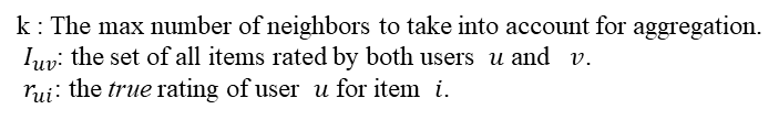
User-based KNNBasic：A basic collaborative filtering algorithm.The prediction 𝑟 ̂ is set as:

The similarity was calculated by MSD, Only common users are taken into account. The Mean Squared Difference is defined as:

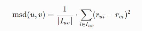
The MSD-similarity is then defined as：

The +1 term is just here to avoid dividing by zero.

of course，you can also use cosine and other similar algorithm，

模型生成

我们使用python 的 surprise library。

代码如下：

#get the data that we define
from surprise import Dataset
from surprise import Reader
reader  = Reader(rating_scale = (1,5))
data = Dataset.load_from_df(ratings[["userId","movieId","rating"]],reader)
rm_data = Dataset.load_from_df(rm_ratings[["userId","movieId","rating"]],reader)

#Compare the accuracy between original data and dealed data
#create model
from surprise import KNNBasic
from surprise.model_selection import cross_validate
sim_options = {
    "name":"MSD",
    'user_based':True
}
knnb = KNNBasic(k=40, min_k=1, sim_options=sim_options, verbose=False)

#using KNNBasic model,computing accuracy metrics on the data and rm_data
result = cross_validate(knnb,data,measures=['RMSE', 'MAE'],cv=5, verbose=True)
rm_result = cross_validate(knnb,rm_data,measures=['RMSE', 'MAE'],cv=5, verbose=True)

#Visaulize RMSE and MAE
fig = plt.figure(dpi = 160,figsize=(5,4)) 
config = {
"font.family":"serif",    #serif
"font.size": 10,
"mathtext.fontset":'stix',
}
rcParams.update(config)
plt.plot(np.arange(1,6),result['test_rmse'], color="y", lw=0.8, ls='-', marker='o', ms=8)
plt.plot(np.arange(1,6),rm_result['test_rmse'], color='green', lw=0.8,  marker='^', ms=8)
plt.xticks([1,2,3,4,5])
# 图例设置
plt.legend(['unprocessed','processed'],loc='best',frameon=False)
plt.ylabel('RMSE')
plt.show()

上图为采用5折交叉验证计算的结果，可见处理后的数据的RMSE更小，推荐系统将更将精确。这是因为我们删除了一部分提供信息很少的users和movies。

调整超参数

我们调整超参数来优化模型：通过改变计算相似度的算法（msd和cosine）以及KNN的k值来调整模型。对于每一个参数点RMSE的计算，我们采用5折交叉验证的平均值来表示
由图可见，在k=20，采用msd算法时，该模型能得到一些性能上的优化。此时模型的RMSE为0.846。

#Adjust the hyperparameter optimization model
from surprise.model_selection import GridSearchCV
param_grid = {'k': np.arange(10,150,10),
              'sim_options': {'name': ['msd', 'cosine'], 
                              'min_support': [1],
                              'user_based': [True]},
              }

gs = GridSearchCV(KNNBasic, param_grid, measures=['rmse', 'mae'], cv=5)
gs.fit(rm_data)
print('best_params:',gs.best_params['rmse'])
print('best score of RMSE:',gs.best_score['rmse'])
grid_result = gs.cv_results['mean_test_rmse']
msd_r = grid_result[np.arange(0,28,2)]
cosin_r = grid_result[np.arange(1,29,2)]
#Visaulize RMSE and MAE for different metrix method
fig = plt.figure(dpi = 160,figsize=(5,4)) 
config = {
"font.family":"serif",    #serif
"font.size": 10,
"mathtext.fontset":'stix',
}
rcParams.update(config)
plt.plot(np.arange(10,150,10),msd_r , color="y", lw=0.8, ls='-', marker='o', ms=8)
plt.plot(np.arange(10,150,10),cosin_r, color='green', lw=0.8,  marker='^', ms=8)
# 图例设置
plt.legend(['msd','cosine'],loc='best',frameon=False)
plt.ylabel('RMSE')
plt.xlabel('K')
plt.show()