信用卡欺诈检测案例

源码下载
信用卡欺诈检测，又叫异常检测。我们可以简单想一下，异常检测无非就是正常和异常，任务一个二分类任务，显然正常的占绝大部分，异常的只占很少的比例，我们要检测的就是这些异常的。明确了我们的任务后，我们要进行二分类的处理了。在Class这列中，0表示正常，1表示异常。

*注意：*第一次使用时需要安装imblearn库。
安装命令：
pip install imblearn
或者使用，选一个就好了
conda install -c glemaitre imbalanced-learn

1.读取数据，数据文件是csv

import pandas as pd
import matplotlib.pyplot as plt
import numpy as np
data = pd.read_csv("creditcard.csv")
data.head(6)

打印结果：

从上我们可以观察到前面有一列时间序列对于我们的异常来说没啥大意义，amount序列数值浮动比较大待会要做标准化或归一化，因为计算机对于数值较大的值会误认为他的权重大，要把数据的大小尽量均衡，class这一列我们可以看到0占的百分比相当高，根据我们前面的分析，0是正常的样本，1为异常的

# 统计Class这一列中有多少不同的值，并排序出来
count_classes = pd.value_counts(data['Class'],sort=True).sort_index()
# 输出结果是：
# 0    284315
# 1       492
# Name: Class, dtype: int64
# print(count_classes)

count_classes.plot(kind='bar')
plt.title("Fraud class histogram")
plt.xlabel("Class")
plt.ylabel("Frequency")
# 绘图
plt.show()

结果：

显然正负样本不均衡，可以通过上下采样调整样本分布均匀。(显然正负样本不均衡，可以通过上下采样调整样本分布均匀)

# 标准化，并产生新的normAmount
# data['normAmount'] = StandardScaler().fit_transform(data['Amount'].reshape(-1, 1)) #错误写法
data['normAmount'] = StandardScaler().fit_transform(data['Amount'].values.reshape(-1, 1))
# 删除无用的所在列
data = data.drop(['Time', 'Amount'], axis=1)
data.head()
# print(data)

结果

注意：很多博客上使用的是
data['normAmount'] = StandardScaler().fit_transform(data['Amount'].reshape(-1, 1))
会出现错误如下:

AttributeError: ‘Series’ object has no attribute ‘reshape’

正确的是data['normAmount'] = StandardScaler().fit_transform(data['Amount'].values.reshape(-1, 1))

下采样数据

# 下采集数据
# 取出所有属性。不包含Class这一列
X = data.ix[:, data.columns != 'Class']
# 另外y=class这一列
y = data.ix[:, data.columns == "Class"]
# 计算出Class这一列中有几个为1的元素
number_record_fraud = len(data[data.Class == 1])
# 取出Class这一列所有等于1的行索引
fraud_indices = np.array(data[data.Class == 1].index)
# 取出Class这一列所有等于0的行索引
normal_indices = np.array(data[data.Class == 0].index)

# 随机选着和1这个属性样本相同个数的0样本
random_normal_indices = np.random.choice(normal_indices, number_record_fraud, replace=False)
# 转换为numpy的格式
random_normal_indices = np.array(random_normal_indices)

# 将正负样本拼接在一起
under_sample_indices = np.concatenate([fraud_indices, random_normal_indices])

# 下采集数据
under_sample_data = data.iloc[under_sample_indices, :]

# 下采集数据集的数据（除Class这列外）
X_undersample = under_sample_data.ix[:, under_sample_data.columns != "Class"]
# 下采集数据集的label（只取Class这列）
y_undersample = under_sample_data.ix[:, under_sample_data.columns == "Class"]

# 输出
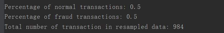
# 打印正样本数目
print("Percentage of normal transactions:",
      len(under_sample_data[under_sample_data.Class == 0]) / len(under_sample_data))
# 打印负样本数目
print("Percentage of fraud transactions:",
      len(under_sample_data[under_sample_data.Class == 1]) / len(under_sample_data))
# 打印总数
print("Total number of transaction in resampled data:",len(under_sample_data))

输出结果：

交叉验证

# 交叉验证模块引入
# from sklearn.cross_validation import train_test_split
from sklearn.model_selection import train_test_split
# 训练集和数据切分
# 对整个训练集进行切分，testsize表示训练集大小，state=0在切分时进行数据重新洗牌的标识位
X_train, X_test, y_train, y_test = train_test_split(X, y, test_size=0.3, random_state=0)

print("Number transactions train dataset:",len(X_train))
print("Number transactions test dataset:",len(X_test))
print("Total number of transactions:",len(X_train)+len(X_test))


# 对下采样数据切分
X_train_undersample,X_test_undersample,y_train_undersample,y_test_undersample=train_test_split(X_undersample,y_undersample,test_size=0.3,random_state=0)
print("切分:")
print("Number transactions train dataset:",len(X_train_undersample))
print("Number transactions test dataset:",len(X_test_undersample))
print("Total number of transactions:",len(X_train_undersample)+len(X_test_undersample))

结果：

注意：引入模块时，from sklearn.cross_validation import train_test_split出现错误：
ModuleNotFoundError: No module named ‘sklearn.cross_validation’

正确引入：from sklearn.model_selection import train_test_split后面有一个需要导入K折交叉验证的模块同理

上面我们可以看到我们制造的样本均衡的数据比较小，在做测试是测试集不足以代表样本的整体性，所以真正测试时还是用原来数据集的测试集比较符合原始数据的分布

可能会出现错误：
解决方法，参考：https://blog.csdn.net/weixin_40283816/article/details/83242777

# 调用逻辑回归模型
from sklearn.linear_model import LogisticRegression
# 调用K折交叉验证
from sklearn.model_selection import KFold, cross_val_score
from sklearn.metrics import confusion_matrix, recall_score, classification_report


# 引用混淆矩阵，召回率
def printing_Kfold_scores(x_train_data, y_train_data):
    # 第一个参数：训练集长度，第二个参数：输入为几折交叉验证
    # from sklearn.model_selection import KFold这个版本的库无需传入总数
    fold = KFold(5, shuffle=False)
    # from sklearn.cross_validation import KFold版本需要传入总数
    # fold = KFold(len(y_train_data), 5, shuffle=False)
    # 传入选择正则化的参数，正则化惩罚项
    c_param_range = [0.01, 0.1, 1, 10, 100]

    results_table = pd.DataFrame(index=range(len(c_param_range), 2), columns=['C_paramter', "Mean recall score"])
    results_table['C_parameter'] = c_param_range

    j = 0
    for c_param in c_param_range:
        print("---------------------------------------")
        print("C parameter:", c_param)
        print("---------------------------------------")
        # 第一个for循环用来了打印每个正则化参数下的输出

        recall_accs = []
        # from sklearn.cross_validation import KFold写法
        # for iteration, indices in enumerate(fold, start=1):
        # from sklearn.model_selection import KFold版本写法；
        for iteration, indices in enumerate(fold.split(x_train_data)):
            # 传入正则化参数下的输出
            # 用一个确定的c参数调用逻辑回归模型，把c_param_range代入到逻辑回归模型中，并使用了l1正则化
            lr = LogisticRegression(C=c_param, penalty='l1', solver='liblinear')
            # 使用训练数据拟合模型，在这个例子中，我们使用这交叉部分训练模型
            # 套路：使训练模型fit模型,使用indices[0]的数据进行拟合曲线，使用indices[1]的数据进行误差测试
            # lr.fit(x_train_data.iloc[indices[0], :], y_train_data.iloc[indices[0], :].values.ravel())
            lr.fit(x_train_data.iloc[indices[0], :], y_train_data.iloc[indices[0], :].values.ravel())
            # 在训练集数据中，使用测试指标来预测值
            y_pred_undersample = lr.predict(x_train_data.iloc[indices[1], :].values)

            # 评估the recall score
            recall_acc = recall_score(y_train_data.iloc[indices[1], :].values, y_pred_undersample)
            recall_accs.append(recall_acc)
            print("Iteration", iteration, ':recall score =', recall_acc)

        # 这些recall scores的平均值，就是我们想要的指标
        results_table.loc[j, 'Mean recall score'] = np.mean(recall_accs)
        j += 1
        print("")
        print("Mean recall score", np.mean(recall_accs))

    best_c = results_table.loc[results_table['Mean recall score'].values.argmax()]['C_parameter']
    # 最后，验证那个c参数是最好的选择
    print("Best model to choose from cross validation is with parameter=", best_c)
    return best_c


best_c = printing_Kfold_scores(X_train_undersample, y_train_undersample)

运行结果

-------------------------------------------
C parameter: 0.1
-------------------------------------------
Iteration 0 : recall score = 0.8356164383561644
Iteration 1 : recall score = 0.863013698630137
Iteration 2 : recall score = 0.9152542372881356
Iteration 3 : recall score = 0.9324324324324325
Iteration 4 : recall score = 0.8939393939393939

Mean recall score 0.8880512401292526

------------------------------------------
C parameter: 1
-------------------------------------------
>Iteration 0 : recall score = 0.8493150684931506
Iteration 1 : recall score = 0.8767123287671232
Iteration 2 : recall score = 0.9661016949152542
Iteration 3 : recall score = 0.9459459459459459
Iteration 4 : recall score = 0.9242424242424242

Mean recall score 0.9124634924727797

-------------------------------------------
C parameter: 10
-------------------------------------------
Iteration 0 : recall score = 0.863013698630137
Iteration 1 : recall score = 0.8767123287671232
Iteration 2 : recall score = 0.9830508474576272
Iteration 3 : recall score = 0.9459459459459459
Iteration 4 : recall score = 0.9242424242424242

Mean recall score 0.9185930490086515

-------------------------------------------
C parameter: 100
-------------------------------------------
Iteration 0 : recall score = 0.863013698630137
Iteration 1 : recall score = 0.8767123287671232
Iteration 2 : recall score = 0.9830508474576272
“the number of iterations.”, ConvergenceWarning)
Iteration 3 : recall score = 0.9459459459459459
Iteration 4 : recall score = 0.9242424242424242


Mean recall score 0.9185930490086515

Best model to choose from cross validation is with C parameter = 0.01

---

混淆矩阵

# 混淆矩阵
import itertools

# 这个方法输出和画出混淆矩阵
def plot_confusion_matrix(cm, classes, title='Confusion matrix', cmap=plt.cm.Blues):
    # cm为数据，interpolation=‘nearest'使用最近邻插值，cmap颜色图谱（colormap），默认绘制为RGB（A）颜色空间
    plt.imshow(cm, interpolation='nearest', cmap=cmap)
    plt.title(title)
    plt.colorbar()
    tick_marks = np.arange(len(classes))
    # xticks为刻度下标
    plt.xticks(tick_marks, classes, rotation=0)
    plt.yticks(tick_marks, classes)
    # text()命令可以在任意位置添加文字
    thresh = cm.max() / 2
    for i, j in itertools.product(range(cm.shape[0]), range(cm.shape[1])):
        plt.text(j, i, cm[i, j], horizontalalignment="center", color="white" if cm[i, j] > thresh else 'black')
    # 自动紧凑布局
    plt.tight_layout()
    plt.ylabel('True label')
    plt.xlabel('Predicted label')

下取样的模型训练与测试

①使用下采样数据训练与测试

lr = LogisticRegression(C=best_c, penalty='l1', solver='liblinear')
lr.fit(X_train_undersample, y_train_undersample.values.ravel())
y_pred_undersample = lr.predict(X_test_undersample.values)
# 计算混淆矩阵
cnf_matrix = confusion_matrix(y_test_undersample, y_pred_undersample)
# 输出精度为小数点后两位
np.set_printoptions(precision=2)
print("Recall metric in the testing dataset:", cnf_matrix[1, 1] / (cnf_matrix[1, 0] + cnf_matrix[1, 1]))
# 画出非标准化的混淆矩阵
class_names = [0, 1]
plt.figure()
plot_confusion_matrix(cnf_matrix, classes=class_names, title='Confusion matrix')
plt.show()

结果

Recall metric in the testing dataset: 0.9319727891156463

②使用下采样数据进行训练，使用原始数据进行测试

# 下采样数据进行训练，使用原始数据进行测试
lr = LogisticRegression(C=best_c,penalty='l1',solver='liblinear')
lr.fit(X_train_undersample,y_train_undersample.values.ravel())
y_pred = lr.predict(X_test.values)
# 计算混淆矩阵
cnf_matrix = confusion_matrix(y_test,y_pred)
# 输出精度为小数点后两位
np.set_printoptions(precision=2)
print("Recall metric in the testing dataset :",cnf_matrix[1,1]/(cnf_matrix[1,0]+cnf_matrix[1,1]))
# 画出非标准化的混淆矩阵
class_names = [0,1]
plt.figure()
plot_confusion_matrix(cnf_matrix,classes=class_names,title='Confusion matrix')
plt.show()

结果

Recall metric in the testing dataset : 0.9115646258503401

说明：对于下采样得到的数据集，虽然召回率比较低，但是误杀还是比较多的。

③原始数据进行K折交叉验证

# 原始数据进行K折交叉验证
best_c = printing_Kfold_scores(X_train, y_train)

结果：

---------------------------------------
C parameter: 0.01
---------------------------------------
Iteration 0 :recall score = 0.4925373134328358 Iteration 1 :recall score = 0.6027397260273972 Iteration 2 :recall score = 0.6833333333333333 Iteration 3 :recall
score = 0.5692307692307692 Iteration 4 :recall score = 0.45 Mean
recall score 0.5595682284048672
---------------------------------------
C parameter: 0.1
---------------------------------------
Iteration 0 :recall score = 0.5671641791044776 Iteration 1 :recall score = 0.6164383561643836 Iteration 2 :recall score = 0.6833333333333333 Iteration 3 :recall
score = 0.5846153846153846 Iteration 4 :recall score = 0.525 Mean
recall score 0.5953102506435158
---------------------------------------
C parameter: 1
---------------------------------------
Iteration 0 :recall score = 0.5522388059701493 Iteration 1 :recall score = 0.6164383561643836 Iteration 2 :recall score = 0.7166666666666667 Iteration 3 :recall
score = 0.6153846153846154 Iteration 4 :recall score = 0.5625 Mean
recall score 0.612645688837163
---------------------------------------
C parameter: 10
---------------------------------------
Iteration 0 :recall score = 0.5522388059701493 Iteration 1 :recall score = 0.6164383561643836 Iteration 2 :recall score = 0.7333333333333333 Iteration 3 :recall
score = 0.6153846153846154 Iteration 4 :recall score = 0.575 Mean
recall score 0.6184790221704963
---------------------------------------
C parameter: 100
---------------------------------------
Iteration 0 :recall score = 0.5522388059701493 Iteration 1 :recall score = 0.6164383561643836 Iteration 2 :recall score = 0.7333333333333333 Iteration 3 :recall
score = 0.6153846153846154 Iteration 4 :recall score = 0.575 Mean
recall score 0.6184790221704963 Best model to choose from cross
validation is with parameter= 10.0

可以看出使用原始数据（不均衡）进行训练的结果召回率很低，因此不建议直接使用原始数据。

④使用原始数据进行训练和测试

# 使用原始数据进行训练与测试
lr = LogisticRegression(C=best_c,penalty='l1',solver='liblinear')
lr.fit(X_train,y_train.values.ravel())
y_pred = lr.predict(X_test.values)
# 计算混淆矩阵
cnf_matrix = confusion_matrix(y_test,y_pred)
# 输出精度为小数点后两位
np.set_printoptions(precision=2)
print("Recall metric in the testing dataset :", cnf_matrix[1, 1] / (cnf_matrix[1, 0] + cnf_matrix[1, 1]))
# 画出非标准化的混淆矩阵
class_names = [0, 1]
plt.figure()
plot_confusion_matrix(cnf_matrix, classes=class_names, title='Confusion matrix')
plt.show()

结果

Recall metric in the testing dataset : 0.6190476190476191

⑤使用下采样数据训练与测试（不同的阈值对结果的影响）

# 使用下采样数据训练与测试（不同的阈值对结果的影响）
lr = LogisticRegression(C=best_c, penalty='l1', solver='liblinear')
lr.fit(X_train_undersample, y_train_undersample.values.ravel())
y_pred_undersample_proba = lr.predict_proba(X_test_undersample.values)
thresholds = [0.1, 0.2, 0.3, 0.4, 0.5, 0.6, 0.7, 0.8, 0.9]
plt.figure(figsize=(10, 10))
j = 1
for i in thresholds:
    y_test_predictions_high_recall = y_pred_undersample_proba[:, 1] > i
    plt.subplot(3, 3, j)
    j += 1
    # 计算混淆矩阵
    cnf_matrix = confusion_matrix(y_test_undersample, y_test_predictions_high_recall)
    # 输出精度为小数点后两位
    np.set_printoptions(precision=2)
    print("Recall metric in the testing dataset:", cnf_matrix[1, 1] / (cnf_matrix[1, 0] + cnf_matrix[1, 1]))
    # 画出非标准化的混淆矩阵
    class_names = [0, 1]
    plot_confusion_matrix(cnf_matrix, classes=class_names, title='Threshold>=%s' % i)
plt.show()

结果：

Recall metric in the testing dataset: 0.9727891156462585
Recall metric in the testing dataset: 0.9523809523809523
Recall metric in the testing dataset: 0.9319727891156463
Recall metric in the testing dataset: 0.9319727891156463
Recall metric in the testing dataset: 0.9319727891156463
Recall metric in the testing dataset: 0.9251700680272109
Recall metric in the testing dataset: 0.8979591836734694
Recall metric in the testing dataset: 0.8775510204081632
Recall metric in the testing dataset: 0.8639455782312925

从以上的实验可以看出，对于阈值，设置的太大不好，设置的太小也不好，所以阈值设定地越适当，才能使得模型拟合效果越好。

---

使用过采样，使得两种样本数据一样多
①SMOTE
AMOTE全称是Synthetic Minority Oversampling Technique,即合成少数过采样技术。
它是基于采样算法的一种改进方案。由于随机采样采取简单素质样本的策略来增加少数类样本，这样容易产生模型过拟合的问题，即是的模型学习到的信息过于特别而不够泛化。
SMOTE算法的基本思想是UID少数类样本进行分析并根据少数类样本人工合成新样本添加到数据集中，

SMOTE算法步骤：

1. 对于少数类中每个样本X，以欧式距离为标准计算它到少数类样本集中所有样本的距离，得到K近邻。
   （如图a，计算Xi到其他样本的距离）
2. 根据样本不平衡比例设置一个采样比例以确定采样倍率N，对于每一个少数类样本X，从其K近邻中随机选择若干个样本，假设选择的近邻为Xn。
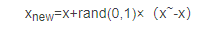
3. 对于每一个随机选出的近邻Xn，分别于原样本安装公式构建新的样本。
   x_new=x+rand(0,1)×（x^~-x）

欧式距离：（样本之间的差异）

如下图所示：

算法流程如下：
设训练的一个少数类样本数为T，那么SMOTE算法将为这个少数类合成NT个新样本。这里要求N必须是正整数，如果给定的N<1，那么算法认为少数类的样本数T=NT，并将强制N=1。
考虑该少数类的一个样本i，其特征向量为xi,i∈{1,…,T}
Step1：首先从该少数类的全部T个样本中找到样本xi的k个近邻（例如欧式距离），记为：xi(near),near∈{1,…,k}
Step2：然后从这k个近邻中随机选择一个样本xi(nn)，再生成一个0到1之间的随机数random，从而合成一个新样本xi1：xi1=xi+random*(xi(nn)-xi)；

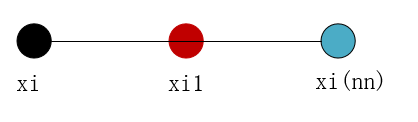
Step3：将步骤2重复进行N次，从而可以合成N个新样本： xinew,new∈{1,…,k}
那么，对全部的T个少数类样本进行上述操作，便可为该少数类合成NT个新样本。
如果样本的特征维数是2维，那么每个样本都可以用二维平面的一个点来表示。SMOTE算法所合成出的一个新样本xi1相当于是表示样本xi的点和表示样本xi(nn)的点之间所连线段上的一个点，所以说该算法是基于“差值”来合成新样本。

②过采样构造数据

import pandas as pd

from imblearn.over_sampling import SMOTE

from sklearn.ensemble import RandomForestClassifier
from sklearn.metrics import confusion_matrix
from sklearn.model_selection import train_test_split

# 读取数据
credit_cards = pd.read_csv('creditcard.csv')
columns = credit_cards.columns
# 为了获得特征列，移除最后一列标签列
features_columns = columns.delete(len(columns) - 1)
features = credit_cards[features_columns]
labels = credit_cards['Class']
features_train, features_test, labels_train, labels_test = train_test_split(features, labels, test_size=0.2,
                                                                            random_state=0)
oversampler = SMOTE(random_state=0)
os_feature, os_labels = oversampler.fit_sample(features_train, labels_train)
print('采样过后，1的样本的个数为：', len(os_labels[os_labels == 1]))

结果：

③K折交叉验证得到最好的C parameter

# K折交叉验证得到最好的C parameter
os_features = pd.DataFrame(os_features)
os_labels = pd.DataFrame(os_labels)
best_c = printing_Kfold_scores(os_features, os_labels)

---------------------------------------
C parameter: 0.01
---------------------------------------
Iteration 0 :recall score = 0.8903225806451613 Iteration 1 :recall score = 0.8947368421052632 Iteration 2 :recall score = 0.968861347792409 Iteration 3 :recall
score = 0.9578043767380002 Iteration 4 :recall score =
0.9584198898671151 Mean recall score 0.9340290074295897
---------------------------------------
C parameter: 0.1
---------------------------------------
Iteration 0 :recall score = 0.8903225806451613 Iteration 1 :recall score = 0.8947368421052632 Iteration 2 :recall score = 0.9701892220869758 Iteration 3 :recall
score = 0.9600246205251646 Iteration 4 :recall score =
0.9601235422780581 Mean recall score 0.9350793615281245
---------------------------------------
C parameter: 1
---------------------------------------
Iteration 0 :recall score = 0.8903225806451613 Iteration 1 :recall score = 0.8947368421052632 Iteration 2 :recall score = 0.9689941352218656 Iteration 3 :recall
score = 0.960310394477968 Iteration 4 :recall score =
0.960530220595509 Mean recall score 0.9349788346091534
---------------------------------------
C parameter: 10
---------------------------------------
Iteration 0 :recall score = 0.8903225806451613 Iteration 1 :recall score = 0.8947368421052632 Iteration 2 :recall score = 0.9709859466637158 Iteration 3 :recall
score = 0.9602224640309516 Iteration 4 :recall score =
0.9608599597718205 Mean recall score 0.9354255586433824
---------------------------------------
C parameter: 100
---------------------------------------
Iteration 0 :recall score = 0.8903225806451613 Iteration 1 :recall score = 0.8947368421052632 Iteration 2 :recall score = 0.9704326657076463 Iteration 3 :recall
score = 0.9596069509018367 Iteration 4 :recall score =
0.9592772117255252 Mean recall score 0.9348752502170864 Best model to choose from cross validation is with parameter= 10.0

④逻辑回归计算混淆矩阵以及召回率

lr = LogisticRegression(C=best_c, penalty='l1', solver='liblinear')
lr.fit(os_features, os_labels.values.ravel())
y_pred = lr.predict(features_test.values)
# 计算混淆矩阵
cnf_matrix = confusion_matrix(labels_test, y_pred)
np.set_printoptions(precision=2)
print("Recall metric in the testing dataset:", cnf_matrix[1, 1] / (cnf_matrix[1, 0] + cnf_matrix[1, 1]))
# 画出非规范化的混淆矩阵
class_names = [0, 1]
plt.figure()
plot_confusion_matrix(cnf_matrix, classes=class_names, title='Confusion matrix')
plt.show()

结果：

Recall metric in the testing dataset: 0.9108910891089109

说明：过采样明显减少了误杀的数量，所以在出现数据不均衡的情况下，较经常使用的是生成数据而不是减少数据，但是数据一旦多起来，运行时间也变长了。

源码下载

参考博客：https://blog.csdn.net/huahuaxiaoshao/article/details/85232089