


一、分类算法
-
逻辑回归
原理


数据User ID Gender Age EstimatedSalary Purchased 15624510 Male 19.0 19000.0 0 15810944 Male 35.0 20000.0 0 15668575 Female 26.0 43000.0 0 15603246 Female 27.0 57000.0 0 15804002 Male 19.0 76000.0 ...import warnings with warnings.catch_warnings(): warnings.filterwarnings("ignore", category=DeprecationWarning) from sklearn.model_selection import train_test_split from sklearn.linear_model import LogisticRegression from sklearn.preprocessing import StandardScaler from sklearn.metrics import confusion_matrix from matplotlib.colors import ListedColormap import matplotlib.pyplot as plt import numpy as np import pandas as pd # Importing the dataset dataset = pd.read_csv('Social_Network_Ads.csv') print(dataset) X = dataset.iloc[:, [2, 3]].values y = dataset.iloc[:, 4].values # Splitting the dataset into the Training set and Test set X_train, X_test, y_train, y_test = train_test_split(X, y, test_size=0.25, random_state=0) # Feature Scaling sc_X = StandardScaler() X_train = sc_X.fit_transform(X_train) X_test = sc_X.transform(X_test) # 分类器 classifier = LogisticRegression(random_state=0) classifier.fit(X_train, y_train) # 预测测试集结果 y_pred = classifier.predict(X_test) # 创建混淆矩阵 cm = confusion_matrix(y_test, y_pred) """ [[65 3] [ 8 24]] 右下对角之和为预测正确的数 左下对角之和为预测错误的数 """ # 画图看效果 # --------------训练集结果------------------- X_set, y_set = X_train, y_train X1, X2 = np.meshgrid(np.arange(start=X_set[:, 0].min() - 1, stop=X_set[:, 0].max() + 1, step=0.01), np.arange(start=X_set[:, 1].min() - 1, stop=X_set[:, 1].max() + 1, step=0.01)) plt.contourf(X1, X2, classifier.predict(np.array([X1.ravel(), X2.ravel()]).T).reshape(X1.shape), alpha=0.75, cmap=ListedColormap(('red', 'green'))) plt.xlim(X1.min(), X1.max()) plt.ylim(X2.min(), X2.max()) for i, j in enumerate(np.unique(y_set)): plt.scatter(X_set[y_set == j, 0], X_set[y_set == j, 1], c=ListedColormap(('orange', 'blue'))(i), label=j) plt.title('Logistic Regression (Training set)') plt.xlabel('Age') plt.ylabel('Estimated Salary') plt.legend() plt.show() X_set, y_set = X_test, y_test X1, X2 = np.meshgrid(np.arange(start=X_set[:, 0].min() - 1, stop=X_set[:, 0].max() + 1, step=0.01), np.arange(start=X_set[:, 1].min() - 1, stop=X_set[:, 1].max() + 1, step=0.01)) plt.contourf(X1, X2, classifier.predict(np.array([X1.ravel(), X2.ravel()]).T).reshape(X1.shape), alpha=0.75, cmap=ListedColormap(('red', 'green'))) plt.xlim(X1.min(), X1.max()) plt.ylim(X2.min(), X2.max()) for i, j in enumerate(np.unique(y_set)): plt.scatter(X_set[y_set == j, 0], X_set[y_set == j, 1], c=ListedColormap(('orange', 'blue'))(i), label=j) plt.title('Logistic Regression (Test set)') plt.xlabel('Age') plt.ylabel('Estimated Salary') plt.legend() plt.show()结果:


-
支持向量机 (SVM)
原理

数据User ID Gender Age EstimatedSalary Purchased 15624510 Male 19.0 19000.0 0 15810944 Male 35.0 20000.0 0 15668575 Female 26.0 43000.0 0 15603246 Female 27.0 57000.0 0 15804002 Male 19.0 76000.0 0 ...import warnings with warnings.catch_warnings(): warnings.filterwarnings("ignore", category=DeprecationWarning) from sklearn.model_selection import train_test_split from sklearn.preprocessing import StandardScaler from sklearn.metrics import confusion_matrix from sklearn.svm import SVC from matplotlib.colors import ListedColormap import matplotlib.pyplot as plt import pandas as pd import numpy as np # Importing the dataset dataset = pd.read_csv('Social_Network_Ads.csv') X = dataset.iloc[:, [2,3]].values y = dataset.iloc[:, 4].values # Splitting the dataset into the Training set and Test set X_train, X_test, y_train, y_test = train_test_split(X, y, test_size = 0.25, random_state = 0) # Feature Scaling sc_X = StandardScaler() X_train = sc_X.fit_transform(X_train) X_test = sc_X.transform(X_test) # Fitting the classifier to the Training set classifier = SVC(kernel="linear", random_state=0) classifier.fit(X_train, y_train) # Predicting the Test set results y_pred = classifier.predict(X_test) # Making the Confusion Matrix cm = confusion_matrix(y_test, y_pred) # Visualising the Training set results X_set, y_set = X_train, y_train X1, X2 = np.meshgrid(np.arange(start=X_set[:, 0].min() - 1, stop=X_set[:, 0].max() + 1, step=0.01), np.arange(start=X_set[:, 1].min() - 1, stop=X_set[:, 1].max() + 1, step=0.01)) plt.contourf(X1, X2, classifier.predict(np.array([X1.ravel(), X2.ravel()]).T).reshape(X1.shape), alpha=0.75, cmap=ListedColormap(('red', 'green'))) plt.xlim(X1.min(), X1.max()) plt.ylim(X2.min(), X2.max()) for i, j in enumerate(np.unique(y_set)): plt.scatter(X_set[y_set == j, 0], X_set[y_set == j, 1], c=ListedColormap(('orange', 'blue'))(i), label=j) plt.title('Classifier (Training set)') plt.xlabel('Age') plt.ylabel('Estimated Salary') plt.legend() plt.show() # Visualising the Test set results X_set, y_set = X_test, y_test X1, X2 = np.meshgrid(np.arange(start=X_set[:, 0].min() - 1, stop=X_set[:, 0].max() + 1, step=0.01), np.arange(start=X_set[:, 1].min() - 1, stop=X_set[:, 1].max() + 1, step=0.01)) plt.contourf(X1, X2, classifier.predict(np.array([X1.ravel(), X2.ravel()]).T).reshape(X1.shape), alpha=0.75, cmap=ListedColormap(('red', 'green'))) plt.xlim(X1.min(), X1.max()) plt.ylim(X2.min(), X2.max()) for i, j in enumerate(np.unique(y_set)): plt.scatter(X_set[y_set == j, 0], X_set[y_set == j, 1], c=ListedColormap(('orange', 'blue'))(i), label=j) plt.title('Classifier (Training set)') plt.xlabel('Age') plt.ylabel('Estimated Salary') plt.legend() plt.show()结果


-
核函数支持向量机 Kernel SVM
Kernel SVM-向高纬度映射


RBF核函数


核函数类型

数据:User ID Gender Age EstimatedSalary Purchased 15624510 Male 19.0 19000.0 0 15810944 Male 35.0 20000.0 0 15668575 Female 26.0 43000.0 0 15603246 Female 27.0 57000.0 0 15804002 Male 19.0 76000.0 0 ...import warnings with warnings.catch_warnings(): warnings.filterwarnings("ignore", category=DeprecationWarning) from sklearn.model_selection import train_test_split from sklearn.preprocessing import StandardScaler from sklearn.metrics import confusion_matrix from sklearn.svm import SVC from matplotlib.colors import ListedColormap import matplotlib.pyplot as plt import numpy as np import pandas as pd # Importing the dataset dataset = pd.read_csv('Social_Network_Ads.csv') X = dataset.iloc[:, [2, 3]].values y = dataset.iloc[:, 4].values # Splitting the dataset into the Training set and Test set X_train, X_test, y_train, y_test = train_test_split(X, y, test_size = 0.25, random_state = 0) # Feature Scaling sc = StandardScaler() X_train = sc.fit_transform(X_train) X_test = sc.transform(X_test) # Fitting classifier to the Training set classifier = SVC(kernel="rbf", random_state=0) # kernel="rbf": 高斯核分类器 classifier = classifier.fit(X_train, y_train) # Predicting the Test set results y_pred = classifier.predict(X_test) # Making the Confusion Matrix cm = confusion_matrix(y_test, y_pred) # Visualising the Training set results X_set, y_set = X_train, y_train X1, X2 = np.meshgrid(np.arange(start=X_set[:, 0].min() - 1, stop=X_set[:, 0].max() + 1, step=0.01), np.arange(start=X_set[:, 1].min() - 1, stop=X_set[:, 1].max() + 1, step=0.01)) plt.contourf(X1, X2, classifier.predict(np.array([X1.ravel(), X2.ravel()]).T).reshape(X1.shape), alpha=0.75, cmap=ListedColormap(('red', 'green'))) plt.xlim(X1.min(), X1.max()) plt.ylim(X2.min(), X2.max()) for i, j in enumerate(np.unique(y_set)): plt.scatter(X_set[y_set == j, 0], X_set[y_set == j, 1], c=ListedColormap(('orange', 'blue'))(i), label=j) plt.title('Classifier (Training set)') plt.xlabel('Age') plt.ylabel('Estimated Salary') plt.legend() plt.show() # Visualising the Test set results X_set, y_set = X_test, y_test X1, X2 = np.meshgrid(np.arange(start=X_set[:, 0].min() - 1, stop=X_set[:, 0].max() + 1, step=0.01), np.arange(start=X_set[:, 1].min() - 1, stop=X_set[:, 1].max() + 1, step=0.01)) plt.contourf(X1, X2, classifier.predict(np.array([X1.ravel(), X2.ravel()]).T).reshape(X1.shape), alpha=0.75, cmap=ListedColormap(('red', 'green'))) plt.xlim(X1.min(), X1.max()) plt.ylim(X2.min(), X2.max()) for i, j in enumerate(np.unique(y_set)): plt.scatter(X_set[y_set == j, 0], X_set[y_set == j, 1], c=ListedColormap(('orange', 'blue'))(i), label=j) plt.title('Classifier (Test set)') plt.xlabel('Age') plt.ylabel('Estimated Salary') plt.legend() plt.show()结果:


-
Naive Bayes(朴素贝叶斯)
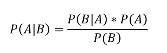
公式
实际用例


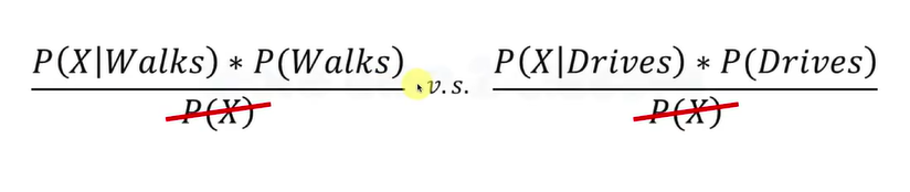
应用示例


数据:User ID Gender Age EstimatedSalary Purchased 15624510 Male 19.0 19000.0 0 15810944 Male 35.0 20000.0 0 15668575 Female 26.0 43000.0 0 15603246 Female 27.0 57000.0 0 15804002 Male 19.0 76000.0 0 ...import warnings with warnings.catch_warnings(): warnings.filterwarnings("ignore", category=DeprecationWarning) from sklearn.model_selection import train_test_split from sklearn.preprocessing import StandardScaler from sklearn.metrics import confusion_matrix from sklearn.naive_bayes import GaussianNB from matplotlib.colors import ListedColormap import matplotlib.pyplot as plt import numpy as np import pandas as pd # Importing the dataset dataset = pd.read_csv('Social_Network_Ads.csv') X = dataset.iloc[:, [2, 3]].values y = dataset.iloc[:, 4].values # Splitting the dataset into the Training set and Test set X_train, X_test, y_train, y_test = train_test_split(X, y, test_size = 0.25, random_state = 0) # Feature Scaling sc = StandardScaler() X_train = sc.fit_transform(X_train) X_test = sc.transform(X_test) # Fitting Naive Bayes to the Training set classifier = GaussianNB() classifier = classifier.fit(X_train, y_train) # Predicting the Test set results y_pred = classifier.predict(X_test) # Making the Confusion Matrix cm = confusion_matrix(y_test, y_pred) # Visualising the Training set results X_set, y_set = X_train, y_train X1, X2 = np.meshgrid(np.arange(start=X_set[:, 0].min() - 1, stop=X_set[:, 0].max() + 1, step=0.01), np.arange(start=X_set[:, 1].min() - 1, stop=X_set[:, 1].max() + 1, step=0.01)) plt.contourf(X1, X2, classifier.predict(np.array([X1.ravel(), X2.ravel()]).T).reshape(X1.shape), alpha=0.75, cmap=ListedColormap(('red', 'green'))) plt.xlim(X1.min(), X1.max()) plt.ylim(X2.min(), X2.max()) for i, j in enumerate(np.unique(y_set)): plt.scatter(X_set[y_set == j, 0], X_set[y_set == j, 1], c=ListedColormap(('orange', 'blue'))(i), label=j) plt.title('Naive Bayes (Training set)') plt.xlabel('Age') plt.ylabel('Estimated Salary') plt.legend() plt.show() # Visualising the Test set results X_set, y_set = X_test, y_test X1, X2 = np.meshgrid(np.arange(start=X_set[:, 0].min() - 1, stop=X_set[:, 0].max() + 1, step=0.01), np.arange(start=X_set[:, 1].min() - 1, stop=X_set[:, 1].max() + 1, step=0.01)) plt.contourf(X1, X2, classifier.predict(np.array([X1.ravel(), X2.ravel()]).T).reshape(X1.shape), alpha=0.75, cmap=ListedColormap(('red', 'green'))) plt.xlim(X1.min(), X1.max()) plt.ylim(X2.min(), X2.max()) for i, j in enumerate(np.unique(y_set)): plt.scatter(X_set[y_set == j, 0], X_set[y_set == j, 1], c=ListedColormap(('orange', 'blue'))(i), label=j) plt.title('Naive Bayes (Test set)') plt.xlabel('Age') plt.ylabel('Estimated Salary') plt.legend() plt.show()结果:


-
Decision Tree Classification(决策树分类器)
原理


数据User ID Gender Age EstimatedSalary Purchased 15624510 Male 19.0 19000.0 0 15810944 Male 35.0 20000.0 0 15668575 Female 26.0 43000.0 0 15603246 Female 27.0 57000.0 0 15804002 Male 19.0 76000.0 0 ...import warnings with warnings.catch_warnings(): warnings.filterwarnings("ignore", category=DeprecationWarning) from sklearn.model_selection import train_test_split from sklearn.preprocessing import StandardScaler from sklearn.tree import DecisionTreeClassifier from sklearn.metrics import confusion_matrix from matplotlib.colors import ListedColormap import matplotlib.pyplot as plt import numpy as np import pandas as pd # Importing the dataset dataset = pd.read_csv('Social_Network_Ads.csv') X = dataset.iloc[:, [2, 3]].values y = dataset.iloc[:, 4].values # Splitting the dataset into the Training set and Test set X_train, X_test, y_train, y_test = train_test_split(X, y, test_size = 0.25, random_state = 0) # # Feature Scaling(若算法中牵扯到欧式距离的运算才进行特征缩放,决策树不需要) sc = StandardScaler() X_train = sc.fit_transform(X_train) X_test = sc.transform(X_test) # Fitting Decision Tree to the Training set classifier = DecisionTreeClassifier(criterion="entropy", random_state=0) classifier = classifier.fit(X_train, y_train) # Predicting the Test set results y_pred = classifier.predict(X_test) # Making the Confusion Matrix cm = confusion_matrix(y_test, y_pred) # Visualising the Training set results X_set, y_set = X_train, y_train X1, X2 = np.meshgrid(np.arange(start=X_set[:, 0].min() - 1, stop=X_set[:, 0].max() + 1, step=0.01), np.arange(start=X_set[:, 1].min() - 1, stop=X_set[:, 1].max() + 1, step=0.01)) plt.contourf(X1, X2, classifier.predict(np.array([X1.ravel(), X2.ravel()]).T).reshape(X1.shape), alpha=0.75, cmap=ListedColormap(('red', 'green'))) plt.xlim(X1.min(), X1.max()) plt.ylim(X2.min(), X2.max()) for i, j in enumerate(np.unique(y_set)): plt.scatter(X_set[y_set == j, 0], X_set[y_set == j, 1], c=ListedColormap(('orange', 'blue'))(i), label=j) plt.title('Decision Tree (Training set)') plt.xlabel('Age') plt.ylabel('Estimated Salary') plt.legend() plt.show() # Visualising the Test set results X_set, y_set = X_test, y_test X1, X2 = np.meshgrid(np.arange(start=X_set[:, 0].min() - 1, stop=X_set[:, 0].max() + 1, step=0.01), np.arange(start=X_set[:, 1].min() - 1, stop=X_set[:, 1].max() + 1, step=0.01)) plt.contourf(X1, X2, classifier.predict(np.array([X1.ravel(), X2.ravel()]).T).reshape(X1.shape), alpha=0.75, cmap=ListedColormap(('red', 'green'))) plt.xlim(X1.min(), X1.max()) plt.ylim(X2.min(), X2.max()) for i, j in enumerate(np.unique(y_set)): plt.scatter(X_set[y_set == j, 0], X_set[y_set == j, 1], c=ListedColormap(('orange', 'blue'))(i), label=j) plt.title('Decision Tree (Test set)') plt.xlabel('Age') plt.ylabel('Estimated Salary') plt.legend() plt.show()结果:


-
Random Forest Classification(随机森林, 和决策树会过渡拟合)
原理

数据:User ID Gender Age EstimatedSalary Purchased 15624510 Male 19.0 19000.0 0 15810944 Male 35.0 20000.0 0 15668575 Female 26.0 43000.0 0 15603246 Female 27.0 57000.0 0 15804002 Male 19.0 76000.0 0 ...import warnings with warnings.catch_warnings(): warnings.filterwarnings("ignore", category=DeprecationWarning) from sklearn.model_selection import train_test_split from sklearn.ensemble import RandomForestClassifier from sklearn.preprocessing import StandardScaler from sklearn.metrics import confusion_matrix from matplotlib.colors import ListedColormap import matplotlib.pyplot as plt import numpy as np import pandas as pd # Importing the dataset dataset = pd.read_csv('Social_Network_Ads.csv') X = dataset.iloc[:, [2, 3]].values y = dataset.iloc[:, 4].values # Splitting the dataset into the Training set and Test set X_train, X_test, y_train, y_test = train_test_split(X, y, test_size = 0.25, random_state = 0) # # Feature Scaling(若算法中牵扯到欧式距离的运算才进行特征缩放,决策树不需要) sc = StandardScaler() X_train = sc.fit_transform(X_train) X_test = sc.transform(X_test) # Fitting Random Forest to the Training set classifier = RandomForestClassifier(n_estimators=10, criterion="entropy", random_state=0) # n_estimators: 决策树的数量 classifier = classifier.fit(X_train, y_train) # Predicting the Test set results y_pred = classifier.predict(X_test) # Making the Confusion Matrix cm = confusion_matrix(y_test, y_pred) # Visualising the Training set results X_set, y_set = X_train, y_train X1, X2 = np.meshgrid(np.arange(start=X_set[:, 0].min() - 1, stop=X_set[:, 0].max() + 1, step=0.01), np.arange(start=X_set[:, 1].min() - 1, stop=X_set[:, 1].max() + 1, step=0.01)) plt.contourf(X1, X2, classifier.predict(np.array([X1.ravel(), X2.ravel()]).T).reshape(X1.shape), alpha=0.75, cmap=ListedColormap(('red', 'green'))) plt.xlim(X1.min(), X1.max()) plt.ylim(X2.min(), X2.max()) for i, j in enumerate(np.unique(y_set)): plt.scatter(X_set[y_set == j, 0], X_set[y_set == j, 1], c=ListedColormap(('orange', 'blue'))(i), label=j) plt.title('Random Forest (Training set)') plt.xlabel('Age') plt.ylabel('Estimated Salary') plt.legend() plt.show() # Visualising the Test set results X_set, y_set = X_test, y_test X1, X2 = np.meshgrid(np.arange(start=X_set[:, 0].min() - 1, stop=X_set[:, 0].max() + 1, step=0.01), np.arange(start=X_set[:, 1].min() - 1, stop=X_set[:, 1].max() + 1, step=0.01)) plt.contourf(X1, X2, classifier.predict(np.array([X1.ravel(), X2.ravel()]).T).reshape(X1.shape), alpha=0.75, cmap=ListedColormap(('red', 'green'))) plt.xlim(X1.min(), X1.max()) plt.ylim(X2.min(), X2.max()) for i, j in enumerate(np.unique(y_set)): plt.scatter(X_set[y_set == j, 0], X_set[y_set == j, 1], c=ListedColormap(('orange', 'blue'))(i), label=j) plt.title('Random Forest (Test set)') plt.xlabel('Age') plt.ylabel('Estimated Salary') plt.legend() plt.show()结果:


二、一些名词概念
-
伪阳性伪阴性

-
累计准确曲线


累计准确曲线-量化评估


 639
639


 被折叠的 条评论
为什么被折叠?
被折叠的 条评论
为什么被折叠?
 到【灌水乐园】发言


