


1. 准备
在之前的工作上增加了韵律的相关特征提取,之前可见:【语音信号处理】1语音信号可视化——时域、频域、语谱图、MFCC详细思路与计算、差分
安装一下这个库:
pip install praat-parselmouth
还有其他的一些,反正缺啥安啥:
pip install pydub
pip install python_speech_features
pip install librosa==0.9
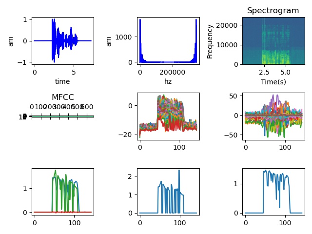
2. 最终结果
3. 代码
"""
This script contains supporting function for the data processing.
It is used in several other scripts:
for generating bvh files, aligning sequences and calculation of speech features
"""

import librosa
import librosa.display

from pydub import AudioSegment # TODO(RN) add dependency!
import parselmouth as pm # TODO(RN) add dependency!
from python_speech_features import mfcc
import scipy.io.wavfile as wav

import numpy as np
import scipy

NFFT = 1024
MFCC_INPUTS=26 # How many features we will store for each MFCC vector
WINDOW_LENGTH = 0.1 #s
SUBSAMPL_RATE = 9

def derivative(x, f):
    """ Calculate numerical derivative (by FDM) of a 1d array
    Args:
        x: input space x
        f: Function of x
    Returns:
        der:  numerical derivative of f wrt x
    """

    x = 1000 * x  # from seconds to milliseconds

    # Normalization:
    dx = (x[1] - x[0])

    cf = np.convolve(f, [1, -1]) / dx

    # Remove unstable values
    der = cf[:-1].copy()
    der[0] = 0

    return der

def create_bvh(filename, prediction, frame_time):
    """
    Create BVH File
    Args:
        filename:    file, in which motion in bvh format should be written
        prediction:  motion sequences, to be written into file
        frame_time:  frame rate of the motion
    Returns:
        nothing, writes motion to the file
    """
    with open('hformat.txt', 'r') as ftemp:
        hformat = ftemp.readlines()

    with open(filename, 'w') as fo:
        prediction = np.squeeze(prediction)
        print("output vector shape: " + str(prediction.shape))
        offset = [0, 60, 0]
        offset_line = "\tOFFSET " + " ".join("{:.6f}".format(x) for x in offset) + '\n'
        fo.write("HIERARCHY\n")
        fo.write("ROOT Hips\n")
        fo.write("{\n")
        fo.write(offset_line)
        fo.writelines(hformat)
        fo.write("MOTION\n")
        fo.write("Frames: " + str(len(prediction)) + '\n')
        fo.write("Frame Time: " + frame_time + "\n")
        for row in prediction:
            row[0:3] = 0
            legs = np.zeros(24)
            row = np.concatenate((row, legs))
            label_line = " ".join("{:.6f}".format(x) for x in row) + " "
            fo.write(label_line + '\n')
        print("bvh generated")


def shorten(arr1, arr2, min_len=0):

    if min_len == 0:
        min_len = min(len(arr1), len(arr2))

    arr1 = arr1[:min_len]
    arr2 = arr2[:min_len]

    return arr1, arr2


def average(arr, n):
    """ Replace every "n" values by their average
    Args:
        arr: input array
        n:   number of elements to average on
    Returns:
        resulting array
    """
    end = n * int(len(arr)/n)
    return np.mean(arr[:end].reshape(-1, n), 1)


def calculate_spectrogram(audio_filename):
    """ Calculate spectrogram for the audio file
    Args:
        audio_filename: audio file name
        duration: the duration (in seconds) that should be read from the file (can be used to load just a part of the audio file)
    Returns:
        log spectrogram values
    """

    DIM = 64

    audio, sample_rate = librosa.load(audio_filename)
    # Make stereo audio being mono
    if len(audio.shape) == 2:
        audio = (audio[:, 0] + audio[:, 1]) / 2

    spectr = librosa.feature.melspectrogram(y=audio, sr=sample_rate, window = scipy.signal.hanning,
                                            #win_length=int(WINDOW_LENGTH * sample_rate),
                                            hop_length = int(WINDOW_LENGTH* sample_rate / 2),
                                            fmax=7500, fmin=100, n_mels=DIM)

    # Shift into the log scale
    eps = 1e-10
    log_spectr = np.log(abs(spectr)+eps)

    return np.transpose(log_spectr)

def calculate_mfcc(audio_filename):
    """
    Calculate MFCC features for the audio in a given file
    Args:
        audio_filename: file name of the audio
    Returns:
        feature_vectors: MFCC feature vector for the given audio file
    """
    fs, audio = wav.read(audio_filename)
    # Make stereo audio being mono
    if len(audio.shape) == 2:
        audio = (audio[:, 0] + audio[:, 1]) / 2

    # Calculate MFCC feature with the window frame it was designed for
    input_vectors = mfcc(audio, winlen=0.02, winstep=0.01, samplerate=fs, numcep=MFCC_INPUTS, nfft=NFFT)

    input_vectors = [average(input_vectors[:, i], 5) for i in range(MFCC_INPUTS)]

    feature_vectors = np.transpose(input_vectors)

    return feature_vectors

def extract_prosodic_features(audio_filename):
    """
    Extract all 5 prosodic features
    Args:
        audio_filename:   file name for the audio to be used
    Returns:
        pros_feature:     energy, energy_der, pitch, pitch_der, pitch_ind
    """

    WINDOW_LENGTH = 5

    # Read audio from file
    sound = AudioSegment.from_file(audio_filename, format="wav")

    # Alternative prosodic features
    pitch, energy = compute_prosody(audio_filename, WINDOW_LENGTH / 1000)

    duration = len(sound) / 1000
    t = np.arange(0, duration, WINDOW_LENGTH / 1000)

    energy_der = derivative(t, energy)
    pitch_der = derivative(t, pitch)

    # Average everything in order to match the frequency
    energy = average(energy, 10)
    energy_der = average(energy_der, 10)
    pitch = average(pitch, 10)
    pitch_der = average(pitch_der, 10)

    # Cut them to the same size
    min_size = min(len(energy), len(energy_der), len(pitch_der), len(pitch_der))
    energy = energy[:min_size]
    energy_der = energy_der[:min_size]
    pitch = pitch[:min_size]
    pitch_der = pitch_der[:min_size]

    # Stack them all together
    pros_feature = np.stack((energy, energy_der, pitch, pitch_der))#, pitch_ind))

    # And reshape
    pros_feature = np.transpose(pros_feature)

    return pros_feature

def compute_prosody(audio_filename, time_step=0.05):
    print(pm.__file__)
    audio = pm.Sound(audio_filename)

    # Extract pitch and intensity
    pitch = audio.to_pitch(time_step=time_step)
    intensity = audio.to_intensity(time_step=time_step)

    # Evenly spaced time steps
    times = np.arange(0, audio.get_total_duration() - time_step, time_step)

    # Compute prosodic features at each time step
    pitch_values = np.nan_to_num(
        np.asarray([pitch.get_value_at_time(t) for t in times]))
    intensity_values = np.nan_to_num(
        np.asarray([intensity.get_value(t) for t in times]))

    intensity_values = np.clip(
        intensity_values, np.finfo(intensity_values.dtype).eps, None)

    # Normalize features [Chiu '11]
    pitch_norm = np.clip(np.log(pitch_values + 1) - 4, 0, None)
    intensity_norm = np.clip(np.log(intensity_values) - 3, 0, None)

    return pitch_norm, intensity_norm


def read_wav(path_wav):
    import wave
    f = wave.open(path_wav, 'rb')
    params = f.getparams()
    nchannels, sampwidth, framerate, nframes = params[:4]  # 通道数、采样字节数、采样率、采样帧数
    voiceStrData = f.readframes(nframes)
    waveData = np.frombuffer(voiceStrData, dtype=np.short)  # 将原始字符数据转换为整数
    waveData = waveData * 1.0 / max(abs(waveData))  # 音频数据归一化, instead of .fromstring
    waveData = np.reshape(waveData, [nframes, nchannels]).T  # .T 表示转置, 将音频信号规整乘每行一路通道信号的格式,即该矩阵一行为一个通道的采样点,共nchannels行
    f.close()
    return waveData, nframes, framerate

import matplotlib.pyplot as plt
def draw_time_domain_image(x1, waveData, nframes, framerate):       # 时域特征
    time = np.arange(0,nframes) * (1.0/framerate)
    # plt.figure(1)
    x1.plot(time,waveData[0,:],c='b')
    plt.xlabel('time')
    plt.ylabel('am')
    # plt.show()


def draw_frequency_domain_image(x2, waveData):      # 频域特征
    fftdata = np.fft.fft(waveData[0, :])
    fftdata = abs(fftdata)
    hz_axis = np.arange(0, len(fftdata))
    # plt.figure(2)
    x2.plot(hz_axis, fftdata, c='b')
    plt.xlabel('hz')
    plt.ylabel('am')
    # plt.show()


def draw_Spectrogram(x3, waveData, framerate):     # 语谱图
    framelength = 0.025     # 帧长20~30ms
    framesize = framelength * framerate       # 每帧点数 N = t*fs,通常情况下值为256或512,要与NFFT相等, 而NFFT最好取2的整数次方,即framesize最好取的整数次方
    nfftdict = {}
    lists = [32, 64, 128, 256, 512, 1024]
    for i in lists:     # 找到与当前framesize最接近的2的正整数次方
        nfftdict[i] = abs(framesize - i)
    sortlist = sorted(nfftdict.items(), key=lambda x: x[1])  # 按与当前framesize差值升序排列
    framesize = int(sortlist[0][0])  # 取最接近当前framesize的那个2的正整数次方值为新的framesize
    NFFT = framesize  # NFFT必须与时域的点数framsize相等,即不补零的FFT
    overlapSize = 1.0 / 3 * framesize  # 重叠部分采样点数overlapSize约为每帧点数的1/3~1/2
    overlapSize = int(round(overlapSize))  # 取整
    spectrum, freqs, ts, fig = x3.specgram(waveData[0], NFFT=NFFT, Fs=framerate, window=np.hanning(M=framesize),
                                            noverlap=overlapSize, mode='default', scale_by_freq=True, sides='default',
                                            scale='dB', xextent=None)  # 绘制频谱图
    plt.ylabel('Frequency')
    plt.xlabel('Time(s)')
    plt.title('Spectrogram')
    # plt.show()


def mfcc_librosa(ax, path):
    y, sr = librosa.load(path, sr=None)
    '''
    librosa.feature.mfcc(y=None, sr=22050, S=None, n_mfcc=20, dct_type=2, norm='ortho', **kwargs)
    y:声音信号的时域序列
    sr:采样频率(默认22050)
    S:对数能量梅尔谱(默认为空)
    n_mfcc:梅尔倒谱系数的数量(默认取20)
    dct_type:离散余弦变换(DCT)的类型(默认为类型2)
    norm:如果DCT的类型为是2或者3,参数设置为"ortho",使用正交归一化DCT基。归一化并不支持DCT类型为1
    kwargs:如果处理时间序列输入,参照melspectrogram
    返回:
    M:MFCC序列
    '''
    mfcc_data = librosa.feature.mfcc(y=y, sr=sr, n_mfcc=13)
    ax.matshow(mfcc_data)
    plt.title('MFCC')
    # plt.show()

from scipy.io import wavfile
from python_speech_features import mfcc, logfbank
def mfcc_python_speech_features(ax, path):
    sampling_freq, audio = wavfile.read(path)       # 读取输入音频文件
    mfcc_features = mfcc(audio, sampling_freq)      # 提取MFCC和滤波器组特征
    filterbank_features = logfbank(audio, sampling_freq)        # numpy.ndarray, (999, 26)
    print(filterbank_features.shape)        # (200, 26)
    print('\nMFCC:\n窗口数 =', mfcc_features.shape[0])
    print('每个特征的长度 =', mfcc_features.shape[1])
    print('\nFilter bank:\n窗口数 =', filterbank_features.shape[0])
    print('每个特征的长度 =', filterbank_features.shape[1])
    mfcc_features = mfcc_features.T     # 画出特征图,将MFCC可视化。转置矩阵,使得时域是水平的
    ax.matshow(mfcc_features)
    plt.title('MFCC')
    filterbank_features = filterbank_features.T     # 将滤波器组特征可视化。转置矩阵,使得时域是水平的
    ax.matshow(filterbank_features)
    plt.title('Filter bank')
    plt.show()


if __name__ == "__main__":
    Debug=1

    if Debug:

        audio_filename = "your path.wav"

        # feature = calculate_spectrogram(audio_filename)


        waveData, nframes, framerate = read_wav(audio_filename)
        ax1 = plt.subplot(3, 3, 1)
        draw_time_domain_image(ax1, waveData, nframes, framerate)
        ax2 = plt.subplot(3, 3, 2)
        draw_frequency_domain_image(ax2, waveData)
        ax3 = plt.subplot(3, 3, 3)
        draw_Spectrogram(ax3, waveData, framerate)
        ax4 = plt.subplot(3, 3, 4)
        mfcc_librosa(ax4, audio_filename)

        x = calculate_spectrogram(audio_filename)
        print(x.shape)      # (145, 64)
        ax5 = plt.subplot(3, 3, 5)
        ax5.plot(x)
        x = calculate_mfcc(audio_filename)
        print(x.shape)      # (143, 26)
        ax6 = plt.subplot(3, 3, 6)
        ax6.plot(x)

        x = extract_prosodic_features(audio_filename)
        print(x.shape)  # (143, 4)
        ax7 = plt.subplot(3, 3, 7)
        ax7.plot(x)

        x, y = compute_prosody(audio_filename, time_step=0.05)
        print(x.shape)  # (143,)
        print(y.shape)  # (143,)
        ax8 = plt.subplot(3, 3, 8)
        ax8.plot(x)
        ax9 = plt.subplot(3, 3, 9)
        ax9.plot(y)
        plt.tight_layout()

        plt.savefig('1.jpg')


 4053
4053


 被折叠的 条评论
为什么被折叠?
被折叠的 条评论
为什么被折叠?
 到【灌水乐园】发言


