


深度学习杂记
step,epoch,batchsize,iteration的区别和联系

随机种子概念(已tf为例)
一.基本理解
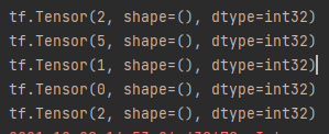
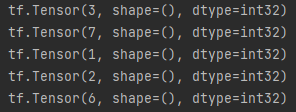
1.随机函数random遵循随机序列去生成随机数,随机序列由全局随机种子和操作种子共通决定,如果都不设置,哪每次生成随机数的时候,随机序列都由系统自选,这会导致同一个代码多次运行的随机数不一致如下图
a = tf.random.uniform(shape=[], maxval=8, dtype=tf.int32)
print(a)
b = tf.random.uniform(shape=[], maxval=8, dtype=tf.int32)
print(b)
c = tf.random.uniform(shape=[], maxval=8, dtype=tf.int32)
print(c)
d = tf.random.uniform(shape=[], maxval=8, dtype=tf.int32)
print(d)
e = tf.random.uniform(shape=[], maxval=8, dtype=tf.int32)
print(e)
执行两次的结果不一致
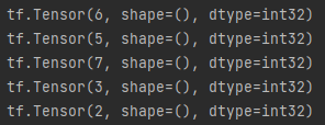
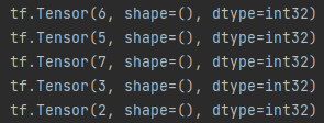
2.当设置了全局种子或操作种子中的一个或两个都设置后,随机序列也就定了,无论执行几次生成的随机数据都是一样的。
tf.random.set_seed(5)
a = tf.random.uniform(shape=[], maxval=8, dtype=tf.int32)
print(a)
b = tf.random.uniform(shape=[], maxval=8, dtype=tf.int32)
print(b)
c = tf.random.uniform(shape=[], maxval=8, dtype=tf.int32)
print(c)
d = tf.random.uniform(shape=[], maxval=8, dtype=tf.int32)
print(d)
e = tf.random.uniform(shape=[], maxval=8, dtype=tf.int32)
print(e)
两次执行结果一致
2.特例
当随机操作在函数中时,函数外多次重启调用,生成的随机数据是不一样的。如果要想使之一样可以使用如下函数定义随机数
tf.random.stateless_uniform(
    shape, seed, minval=0, maxval=None, dtype=tf.dtypes.float32, name=None,
    alg='auto_select'
)
tf张量的定义和np数据的转换
tf张量的定义
张量有三种,常量,变量,占位符(不需要初始化的变量)
常张量
tf.constant(
    value, dtype=None, shape=None, name='Const'
)
变张量
tf.Variable(
    initial_value=None, trainable=None, validate_shape=True, caching_device=None,
    name=None, variable_def=None, dtype=None, import_scope=None, constraint=None,
    synchronization=tf.VariableSynchronization.AUTO,
    aggregation=tf.compat.v1.VariableAggregation.NONE, shape=None
)
name_varible = tf.Variable(initial_value=(5,20),shape=(2,))
print(name_varible)
name_varible.assign([10,60])
print(name_varible)
执行结果
<tf.Variable 'Variable:0' shape=(2,) dtype=int32, numpy=array([ 5, 20])>
<tf.Variable 'Variable:0' shape=(2,) dtype=int32, numpy=array([10, 60])>
tensor张量转numpy
tensor数据自带转换np的方法
a = tf.constant([[1.0, 2.0], [3.0, 4.0]])
print(a.numpy())
张量和np数据都可以作为彼此函数或算子的输入参数
a = tf.constant([[1, 2, 3], [4, 5, 6]])
b = np.array([[1, 2, 3], [4, 5, 6]])
c = tf.add(a,b)
d = np.add(a,b)
print(c,"\n",d)
tf.Tensor(
[[ 2  4  6]
 [ 8 10 12]], shape=(2, 3), dtype=int32)
 [[ 2  4  6]
 [ 8 10 12]]
神经网络正向传播和反向传播的理解
网络间的数据传播与矫正分为三步
1.输入的x数据经过神经元的权重(w)和偏置(b)所进行的矩阵计算,我们假定他的计算结果输出是z,
z
=
w
x
+
b
z = wx+b
z=wx+b
2.上一步的z需要经过激活函数,这边的y简单理解就是网络的预测值
y
=
σ
(
z
)
y=\sigma(z)
y=σ(z)
3.损失函数loss,(其实就是用各种公式去比较网络的输出和实际输出,最简单的就是标准差)
l
o
s
s
=
l
(
y
)
loss = l(y)
loss=l(y)
常见的损失函数
正向传播
经过上面的前两步就可以出结果
反向传播
最终的目的是让偏导结果趋于0
∂
(
l
o
s
s
)
∂
(
w
)
=
∂
(
l
o
s
s
)
∂
(
y
)
∗
∂
(
y
)
∂
(
z
)
∗
∂
(
z
)
∂
(
w
)
\frac{\partial (loss) }{\partial (w)}= \frac{\partial (loss) }{\partial (y)}*\frac{\partial (y) }{\partial (z)}*\frac{\partial (z) }{\partial (w)}
∂(w)∂(loss)=∂(y)∂(loss)∗∂(z)∂(y)∗∂(w)∂(z)
正好对应上面说的三个部分,对损失函数的偏导,对激发函数的偏导,对矩阵计算的偏导
根据数学知识,在已知实际y和预测y的前提下,因为是对单一w求偏导,其他w都视为常量,可以把偏导目标简化为一次函数
l
o
s
s
(
w
)
=
k
w
+
b
loss(w) = kw+b
loss(w)=kw+b
这样理解的话就是
偏导结果k>0,w的函数增,且loss>0,w要尽量的小,loss才能向0收敛
偏导结果k<0,w的函数减,且loss>0,w要尽量的大,loss才能向0收敛
w的更新,引出学习率a (a>0)
w
=
w
+
a
∗
Δ
w
w = w +a*\Delta w
w=w+a∗Δw
激活函数
1.tanh和sigmoid随着自变量变大,导数趋于0,
2.relu小于0的部分,存在数据损失。
1.常见激活函数的图形(relu,sogmoid,tanh,。。。)
import math
import numpy as np


# 做一些假数据来观看图像
x_np = np.arange(-10, 10, 0.1)
x = np.arange(-10, 10, 0.1)

# 几种常用的 激励函数
y_relu = np.where(x < 0, 0, x)
y_sigmoid = 1 / (1 + math.e ** (-x))
y_tanh = (math.e ** (x) - math.e ** (-x)) / (math.e ** (x) + math.e ** (-x))

y_relu_d = np.where(x < 0, 0, 1)
y_sigmoid_d = 1 / (2 + math.e ** (-x)+ math.e ** (x))
y_tanh_d = 1-y_tanh*y_tanh
# y_softmax = F.softmax(x)  softmax 比较特殊, 不能直接显示, 不过他是关于概率的, 用于分类

import matplotlib.pyplot as plt

plt.figure(1, figsize=(8, 6))
plt.axis('on')
plt.subplot(221)
plt.plot(x_np, y_relu, c='red', label='relu')
plt.plot(x_np, y_relu_d, c='blue', label='relu_d')
plt.ylim((-1, 10))
plt.legend(loc='best')

plt.subplot(222)
plt.plot(x_np, y_sigmoid, c='red', label='sigmoid')
plt.plot(x_np, y_sigmoid_d, c='blue', label='sigmoid_d')
plt.ylim((-0.2, 1.2))
plt.legend(loc='best')

plt.subplot(223)
plt.plot(x_np, y_tanh, c='red', label='tanh')
plt.plot(x_np, y_tanh_d, c='blue', label='tanh_d')
plt.ylim((-1.2, 1.2))
plt.legend(loc='best')

# plt.subplot(224)
# plt.plot(x_np, y_softplus, c='red', label='softplus')
# plt.ylim((-0.2, 6))
# plt.legend(loc='best')

plt.show()


 447
447


 被折叠的 条评论
为什么被折叠?
被折叠的 条评论
为什么被折叠?
 到【灌水乐园】发言


