


一、GammaTone 滤波器详解
定义:
外界语音信号进入耳蜗的基底膜后,将依据频率进行分解并产生行波震动,从而刺激听觉感受细胞[1]。GammaTone 滤波器是一组用来模拟耳蜗频率分解特点的滤波器模型,可以用于音频信号的分解,便于后续进行特征提取。
历史:
一般认为外周听觉系统的频率分析方式可以通过一组带通滤波器来进行一定程度的模拟,人们为此也提出了各种各样的滤波器组,如 roex 滤波器(Patterson and Moore 1986)。
在神经科学上有一种叫做反向相关性 “reverse correlation”(de Boer and Kuyper 1968)的计算方式,通过计算初级听觉神经纤维对于白噪声刺激的响应以及相关程度,即听觉神经元发放动作电位前的平均叠加信号,从而直接从生理状态上估计听觉滤波器的形状。这个滤波器是在外周听觉神经发放动作电位前生效的,因此得名为“revcor function”,可以作为一定限度下对外周听觉滤波器冲激响应的估计,也就是耳蜗等对音频信号的前置带通滤波。
GammaTone滤波器(GTF)是一个用来逼近 recvor function 的数学解析式,是 Johannesma 在1972年提出的。这个滤波器组有着简单的数学表达形式,能够很方便地解析到它的各种特性。由于GTF是从冲激响应的测量中得到的,因此它有完整的幅度和相位信息,相比之下,心理声学屏蔽实验中也就只能测得单一的幅度信息,譬如 roex 滤波器。
Holdsworth 等人(1988)进一步阐明了GTF的各种特性,而且提供了一个数字IIR滤波器设计方案。这个技术使得GTF能够比FIR更加容易且高效地实现,为后续出现一些重要的实际应用做了铺垫(Patterson 1988)。[2]
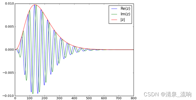
时域表达式:
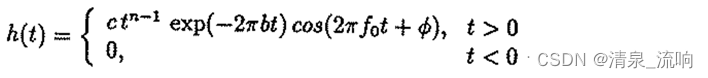
c为比例系数;n为滤波器阶数,越大则偏度越低,滤波器越“瘦高”;b是时间衰减系数,越大则滤波时间越短;f0是滤波器中心频率;Φ是滤波器相位。
频域表达式:
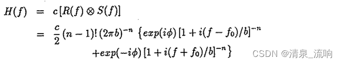
频率表达式中 R(f) 是 指数+阶跃函数的傅里叶变换,阶跃函数用来区别 t>0 和 t<0
S(f) 是频率为 f0 的余弦的傅里叶变换。
可以看到是一个中心频率在 f0 、 在两侧按照e指数衰减的滤波器。
通过上述表达式可以生成一组滤波器:
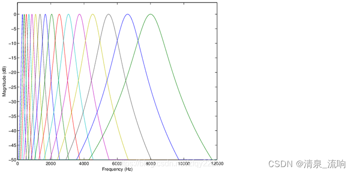
可以看到低频段分得很细,高频段分得很粗,和人耳听觉特性较为符合。
二、GammaTone 滤波器MATLAB实现
MakeERBFilters函数产生了GT滤波器系数。输入为:采样频率、滤波器通道数、最小频率。输出为:fcoefs为n个通道GT滤波器系数;cf为滤波器组的各个中心频率。代码如下:
function [fcoefs,cf]=MakeERBFilters(fs,numChannels,lowFreq)
%获取GT滤波器系数。输入为:采样频率、滤波器通道数、最小频率。
%输出:fcoefs为n个通道GT滤波器系数;cf为滤波器组的各个中心频率。
% function [fcoefs,cf]=MakeERBFilters(fs,numChannels,lowFreq)
% This function computes the filter coefficients for a bank of
% Gammatone filters.  These filters were defined by Patterson and
% Holdworth for simulating the cochlea.
% 这个函数计算一组伽玛通滤波器的滤波系数。这些滤波器是由Patterson和Holdworth为模拟耳蜗而定义的。
% The result is returned as an array of filter coefficients.  Each row
% of the filter arrays contains the coefficients for four second order
% filters.  The transfer function for these four filters share the same
% denominator (poles) but have different numerators (zeros).  All of these
% coefficients are assembled into one vector that the ERBFilterBank
% can take apart to implement the filter.
%结果以过滤器系数数组的形式返回。滤波器阵列的每一行都包含四个二阶滤波器的系数。这四个滤波器的传递函数有相同的分母(极点),
%但有不同的分子(零)。所有这些系数被组合成一个向量,ERBFilterBank可以分解它来实现过滤器。
% The filter bank contains "numChannels" channels that extend from
% half the sampling rate (fs) to "lowFreq".  Alternatively, if the numChannels
% input argument is a vector, then the values of this vector are taken to
% be the center frequency of each desired filter.  (The lowFreq argument is
% ignored in this case.)
%滤波器组包含“numChannels”通道,从采样率(fs)的一半扩展到“lowFreq”。或者,如果numChannels输入参数
%是一个向量,那么这个向量的值被当作每个期望滤波器的中心频率。(lowFreq参数在这种情况下被忽略。)
% Note this implementation fixes a problem in the original code by
% computing four separate second order filters.  This avoids a big
% problem with round off errors in cases of very small cfs (100Hz) and
% large sample rates (44kHz).  The problem is caused by roundoff error
% when a number of poles are combined, all very close to the unit
% circle.  Small errors in the eigth order coefficient, are multiplied
% when the eigth root is taken to give the pole location.  These small
% errors lead to poles outside the unit circle and instability.  Thanks
% to Julius Smith for leading me to the proper explanation.
%注意,这个实现通过计算四个独立的二阶滤波器解决了原始代码中的一个问题。
%在cfs非常小(100Hz)和大样本率(44kHz)的情况下,这避免了舍入误差的大问题。
%这个问题是由舍入误差引起的,当许多极点结合在一起,都非常接近单位圆。八阶系数的小误差,
%乘上八根给出极点位置。这些小误差导致极点在单位圆外而不稳定。感谢朱利叶斯·史密斯给我正确的解释。
% Execute the following code to evaluate the frequency
% response of a 10 channel filterbank.
%执行以下代码来评估10通道滤波器组的频率响应。
%	fcoefs = MakeERBFilters(16000,10,100);
%	y = ERBFilterBank([1 zeros(1,511)], fcoefs);
%	resp = 20*log10(abs(fft(y')));
%	freqScale = (0:511)/512*16000;
%	semilogx(freqScale(1:255),resp(1:255,:));
%	axis([100 16000 -60 0])
%	xlabel('Frequency (Hz)'); ylabel('Filter Response (dB)');

% Rewritten by Malcolm Slaney@Interval.  June 11, 1998.
% (c) 1998 Interval Research Corporation

T = 1/fs;
if length(numChannels) == 1
	cf = ERBSpace(lowFreq, fs/2, numChannels);
else
	cf = numChannels(1:end);
	if size(cf,2) > size(cf,1)
		cf = cf';
	end
end

% Change the following three parameters if you wish to use a different
% ERB scale.  Must change in ERBSpace too.
%如果您希望使用不同的ERB刻度,请更改以下三个参数。在ERBSpace中也必须更改。
EarQ = 9.26449;				%  Glasberg and Moore Parameters
minBW = 24.7;
order = 1;

ERB = ((cf/EarQ).^order + minBW^order).^(1/order);
B=1.019*2*pi*ERB;

A0 = T;
A2 = 0;
B0 = 1;
B1 = -2*cos(2*cf*pi*T)./exp(B*T);
B2 = exp(-2*B*T);

A11 = -(2*T*cos(2*cf*pi*T)./exp(B*T) + 2*sqrt(3+2^1.5)*T*sin(2*cf*pi*T)./ ...
		exp(B*T))/2;
A12 = -(2*T*cos(2*cf*pi*T)./exp(B*T) - 2*sqrt(3+2^1.5)*T*sin(2*cf*pi*T)./ ...
		exp(B*T))/2;
A13 = -(2*T*cos(2*cf*pi*T)./exp(B*T) + 2*sqrt(3-2^1.5)*T*sin(2*cf*pi*T)./ ...
		exp(B*T))/2;
A14 = -(2*T*cos(2*cf*pi*T)./exp(B*T) - 2*sqrt(3-2^1.5)*T*sin(2*cf*pi*T)./ ...
		exp(B*T))/2;

gain = abs((-2*exp(4*i*cf*pi*T)*T + ...
                 2*exp(-(B*T) + 2*i*cf*pi*T).*T.* ...
                         (cos(2*cf*pi*T) - sqrt(3 - 2^(3/2))* ...
                          sin(2*cf*pi*T))) .* ...
           (-2*exp(4*i*cf*pi*T)*T + ...
             2*exp(-(B*T) + 2*i*cf*pi*T).*T.* ...
              (cos(2*cf*pi*T) + sqrt(3 - 2^(3/2)) * ...
               sin(2*cf*pi*T))).* ...
           (-2*exp(4*i*cf*pi*T)*T + ...
             2*exp(-(B*T) + 2*i*cf*pi*T).*T.* ...
              (cos(2*cf*pi*T) - ...
               sqrt(3 + 2^(3/2))*sin(2*cf*pi*T))) .* ...
           (-2*exp(4*i*cf*pi*T)*T + 2*exp(-(B*T) + 2*i*cf*pi*T).*T.* ...
           (cos(2*cf*pi*T) + sqrt(3 + 2^(3/2))*sin(2*cf*pi*T))) ./ ...
          (-2 ./ exp(2*B*T) - 2*exp(4*i*cf*pi*T) +  ...
           2*(1 + exp(4*i*cf*pi*T))./exp(B*T)).^4);

allfilts = ones(length(cf),1);
fcoefs = [A0*allfilts A11 A12 A13 A14 A2*allfilts B0*allfilts B1 B2 gain];

if (0)						% Test Code
	A0  = fcoefs(:,1);
	A11 = fcoefs(:,2);
	A12 = fcoefs(:,3);
	A13 = fcoefs(:,4);
	A14 = fcoefs(:,5);
	A2  = fcoefs(:,6);
	B0  = fcoefs(:,7);
	B1  = fcoefs(:,8);
	B2  = fcoefs(:,9);
	gain= fcoefs(:,10);
	chan=1;
	x = [1 zeros(1, 511)];
	y1=filter([A0(chan)/gain(chan) A11(chan)/gain(chan) ...
		A2(chan)/gain(chan)],[B0(chan) B1(chan) B2(chan)], x);
	y2=filter([A0(chan) A12(chan) A2(chan)], ...
			[B0(chan) B1(chan) B2(chan)], y1);
	y3=filter([A0(chan) A13(chan) A2(chan)], ...
			[B0(chan) B1(chan) B2(chan)], y2);
	y4=filter([A0(chan) A14(chan) A2(chan)], ...
			[B0(chan) B1(chan) B2(chan)], y3);
	semilogx((0:(length(x)-1))*(fs/length(x)),20*log10(abs(fft(y4))));
end
ERBSpace函数获得了中心频率f。输入为:最小频率、最大频率、滤波器通道数。输出为滤波器组的各个中心频率。代码如下:
function cfArray = ERBSpace(lowFreq, highFreq, N)
%功能,获取信号的中心频率
%输入为:最小频率、最大频率、滤波器通道数。输出为滤波器组的各个中心频率。
% function cfArray = ERBSpace(lowFreq, highFreq, N)
%这个函数计算在ERB尺度上均匀间隔在高频率和低频率之间的N个频率的数组。如果未指定N,则设置为100。
% This function computes an array of N frequencies uniformly spaced between
% highFreq and lowFreq on an ERB scale.  N is set to 100 if not specified.
%参见linspace, logspace, MakeERBCoeffs, MakeERBFilters。
% See also linspace, logspace, MakeERBCoeffs, MakeERBFilters.
%关于ERB的定义,请参阅Moore, b.c.j和Glasberg, b.r.(1983)。
%计算听觉滤波器带宽和激发模式的建议公式,J. Acoust。Soc。。74年,750 - 753。
% For a definition of ERB, see Moore, B. C. J., and Glasberg, B. R. (1983).
% "Suggested formulae for calculating auditory-filter bandwidths and
% excitation patterns," J. Acoust. Soc. Am. 74, 750-753.

if nargin < 1
	lowFreq = 100;
end

if nargin < 2
	highFreq = 44100/4;
end

if nargin < 3
	N = 100;
end
%如果您希望使用不同的ERB刻度,请更改以下三个参数。在MakeERBCoeffs中也必须更改。
% Change the following three parameters if you wish to use a different
% ERB scale.  Must change in MakeERBCoeffs too.
EarQ = 9.26449;				%  Glasberg and Moore Parameters
minBW = 24.7;
order = 1;

% All of the followFreqing expressions are derived in Apple TR #35, "An
% Efficient Implementation of the Patterson-Holdsworth Cochlear
% Filter Bank."  See pages 33-34.
cfArray = -(EarQ*minBW) + exp((1:N)'*(-log(highFreq + EarQ*minBW) + ...
		log(lowFreq + EarQ*minBW))/N) * (highFreq + EarQ*minBW);
ERBFilterBank 函数输入分别为:原始数据和GT滤波器系数,GT滤波器系数由MakeERBFilters函数获得。输出为滤波后的数据。该函数实现对原始数据的时域GT滤波。代码如下:
function output = ERBFilterBank(x, fcoefs)
%输入分别为:原始数据和GT滤波器系数。输出为滤波后的数据。该函数实现对原始数据的时域GT滤波。
%GT滤波器系数由MakeERBFilters函数获得
% function output = ERBFilterBank(x, fcoefs)
%用伽马通滤波器组处理输入波形。这个函数接受单个声音矢量,并返回一个滤波器输出数组,每行一个声道。
% Process an input waveform with a gammatone filter bank. This function
% takes a single sound vector, and returns an array of filter outputs, one
% channel per row.
%fcoefs参数完全指定Gammatone滤波器组,应该使用MakeERBFilters函数来设计。如果省略了它,
%则假设22050Hz采样率和64个按ERB尺度从fs/2到100Hz规则间隔的滤波器系数将为您计算。
% The fcoefs parameter, which completely specifies the Gammatone filterbank,
% should be designed with the MakeERBFilters function.  If it is omitted,
% the filter coefficients are computed for you assuming a 22050Hz sampling
% rate and 64 filters regularly spaced on an ERB scale from fs/2 down to 100Hz.
%

% Malcolm Slaney @ Interval, June 11, 1998.
% (c) 1998 Interval Research Corporation
% Thanks to Alain de Cheveigne' for his suggestions and improvements.

if nargin < 1
	error('Syntax: output_array = ERBFilterBank(input_vector[, fcoefs]);');
end

if nargin < 2
	fcoefs = MakeERBFilters(22050,64,100);
end

if size(fcoefs,2) ~= 10
	error('fcoefs parameter passed to ERBFilterBank is the wrong size.');
end

if size(x,2) < size(x,1)
	x = x';
end

A0  = fcoefs(:,1);
A11 = fcoefs(:,2);
A12 = fcoefs(:,3);
A13 = fcoefs(:,4);
A14 = fcoefs(:,5);
A2  = fcoefs(:,6);
B0  = fcoefs(:,7);
B1  = fcoefs(:,8);
B2  = fcoefs(:,9);
gain= fcoefs(:,10);

output = zeros(size(gain,1), length(x));
for chan = 1: size(gain,1)
	y1=filter([A0(chan)/gain(chan) A11(chan)/gain(chan) ...
		   A2(chan)/gain(chan)], ...
				[B0(chan) B1(chan) B2(chan)], x);
	y2=filter([A0(chan) A12(chan) A2(chan)], ...
				[B0(chan) B1(chan) B2(chan)], y1);
	y3=filter([A0(chan) A13(chan) A2(chan)], ...
				[B0(chan) B1(chan) B2(chan)], y2);
	y4=filter([A0(chan) A14(chan) A2(chan)], ...
				[B0(chan) B1(chan) B2(chan)], y3);
	output(chan, :) = y4;
end

if 0
	semilogx((0:(length(x)-1))*(fs/length(x)),20*log10(abs(fft(output))));
end
fft2gammatonemx为获得了GT滤波器的频率域系数。输入为:滤波器长度、采样频率、滤波器通道数、滤波器带宽、最小频率、最大频率、最大长度。输出为GT滤波器的频率域系数。代码如下:
function [wts,gain] = fft2gammatonemx(nfft, sr, nfilts, width, minfreq, maxfreq, maxlen)
%获得GT滤波器的频率域系数。
%输入为:滤波器长度、采样频率、滤波器通道数、滤波器带宽、最小频率、最大频率、最大长度。
%输出为GT滤波器的频率域系数。
% wts = fft2gammatonemx(nfft, sr, nfilts, width, minfreq, maxfreq, maxlen)
%      Generate a matrix of weights to combine FFT bins into
%      Gammatone bins.  nfft defines the source FFT size at
%      sampling rate sr.  Optional nfilts specifies the number of
%      output bands required (default 64), and width is the
%      constant width of each band in Bark (default 1).
%      minfreq, maxfreq specify range covered in Hz (100, sr/2).
%      While wts has nfft columns, the second half are all zero.
%      Hence, aud spectrum is
%      fft2gammatonemx(nfft,sr)*abs(fft(xincols,nfft));
%      maxlen truncates the rows to this many bins
%生成一个权重矩阵,将FFT容器组合成Gammatone容器。nfft定义采样率sr时源FFT大小。
%可选的nfilts指定所需的输出频带数(默认64),width是Bark中每个频带的恒定宽度(默认1)。
%minfreq, maxfreq指定Hz覆盖范围(100,sr/2)。虽然wts有nfft列,但后半部分都是零。
%因此,aud频谱为fft2gammatonemx(nfft,sr)*abs(fft(xincols,nfft));Maxlen将行截断到这么多的容器中
% 2004-09-05  Dan Ellis dpwe@ee.columbia.edu  based on rastamat/audspec.m
% Last updated: $Date: 2009/02/22 02:29:25 $

if nargin < 2;    sr = 16000; end
if nargin < 3;    nfilts = 64; end
if nargin < 4;    width = 1.0; end
if nargin < 5;    minfreq = 100; end
if nargin < 6;    maxfreq = sr/2; end
if nargin < 7;    maxlen = nfft; end

wts = zeros(nfilts, nfft);

% after Slaney's MakeERBFilters
EarQ = 9.26449;
minBW = 24.7;
order = 1;

cfreqs = -(EarQ*minBW) + exp((1:nfilts)'*(-log(maxfreq + EarQ*minBW) + ...
                log(minfreq + EarQ*minBW))/nfilts) * (maxfreq + EarQ*minBW);
cfreqs = flipud(cfreqs);

GTord = 4;

ucirc = exp(j*2*pi*[0:(nfft/2)]/nfft);

justpoles = 0;

for i = 1:nfilts
  cf = cfreqs(i);
  ERB = width*((cf/EarQ).^order + minBW^order).^(1/order);
  B = 1.019*2*pi*ERB;
  r = exp(-B/sr);
  theta = 2*pi*cf/sr;
  pole = r*exp(j*theta);

  if justpoles == 1
    % point on unit circle of maximum gain, from differentiating magnitude
    cosomegamax = (1+r*r)/(2*r)*cos(theta);
    if abs(cosomegamax) > 1
      if theta < pi/2;  omegamax = 0;
      else              omegamax = pi;   end
    else
      omegamax = acos(cosomegamax);
    end
    center = exp(j*omegamax);
    gain = abs((pole-center).*(pole'-center)).^GTord;
    wts(i,1:(nfft/2+1)) = gain * (abs((pole-ucirc).*(pole'- ...
                                                     ucirc)).^-GTord);
  else
    % poles and zeros, following Malcolm's MakeERBFilter
    T = 1/sr;
    A11 = -(2*T*cos(2*cf*pi*T)./exp(B*T) + 2*sqrt(3+2^1.5)*T*sin(2* ...
                                                      cf*pi*T)./exp(B*T))/2;
    A12 = -(2*T*cos(2*cf*pi*T)./exp(B*T) - 2*sqrt(3+2^1.5)*T*sin(2* ...
                                                      cf*pi*T)./exp(B*T))/2;
    A13 = -(2*T*cos(2*cf*pi*T)./exp(B*T) + 2*sqrt(3-2^1.5)*T*sin(2* ...
                                                      cf*pi*T)./exp(B*T))/2;
    A14 = -(2*T*cos(2*cf*pi*T)./exp(B*T) - 2*sqrt(3-2^1.5)*T*sin(2* ...
                                                      cf*pi*T)./exp(B*T))/2;
    zros = -[A11 A12 A13 A14]/T;

    gain(i) =  abs((-2*exp(4*j*cf*pi*T)*T + ...
                2*exp(-(B*T) + 2*j*cf*pi*T).*T.* ...
                (cos(2*cf*pi*T) - sqrt(3 - 2^(3/2))* ...
                 sin(2*cf*pi*T))) .* ...
               (-2*exp(4*j*cf*pi*T)*T + ...
                2*exp(-(B*T) + 2*j*cf*pi*T).*T.* ...
                (cos(2*cf*pi*T) + sqrt(3 - 2^(3/2)) * ...
                 sin(2*cf*pi*T))).* ...
               (-2*exp(4*j*cf*pi*T)*T + ...
                2*exp(-(B*T) + 2*j*cf*pi*T).*T.* ...
                (cos(2*cf*pi*T) - ...
                 sqrt(3 + 2^(3/2))*sin(2*cf*pi*T))) .* ...
               (-2*exp(4*j*cf*pi*T)*T + 2*exp(-(B*T) + 2*j*cf*pi*T).*T.* ...
                (cos(2*cf*pi*T) + sqrt(3 + 2^(3/2))*sin(2*cf*pi*T))) ./ ...
               (-2 ./ exp(2*B*T) - 2*exp(4*j*cf*pi*T) +  ...
                2*(1 + exp(4*j*cf*pi*T))./exp(B*T)).^4);
    wts(i,1:(nfft/2+1)) = ((T^4)/gain(i)) ...
        * abs(ucirc-zros(1)).*abs(ucirc-zros(2))...
        .*abs(ucirc-zros(3)).*abs(ucirc-zros(4))...
        .*(abs((pole-ucirc).*(pole'-ucirc)).^-GTord);
  end
end

wts = wts(:,1:maxlen);
specgram函数是计算和线索频谱图,程序如下:
function y = specgram(x,n,sr,w,ov)
% Y = myspecgram(X,NFFT,SR,W,OV)
%代替Matlab的谱图,计算和显示谱图
%      Substitute for Matlab's specgram, calculates & displays spectrogram
% $Header: /homes/dpwe/tmp/e6820/RCS/myspecgram.m,v 1.1 2002/08/04 19:20:27 dpwe Exp $

if (size(x,1) > size(x,2))
  x = x';
end

s = length(x);

if nargin < 2
  n = 256;
end
if nargin < 3
  sr = 1;
end
if nargin < 4
  w = n;
end
if nargin < 5
  ov = w/2;
end
h = w - ov;

halflen = w/2;
halff = n/2;   % midpoint of win
acthalflen = min(halff, halflen);

halfwin = 0.5 * ( 1 + cos( pi * (0:halflen)/halflen));
win = zeros(1, n);
win((halff+1):(halff+acthalflen)) = halfwin(1:acthalflen);
win((halff+1):-1:(halff-acthalflen+2)) = halfwin(1:acthalflen);

c = 1;

% pre-allocate output array
ncols = 1+fix((s-n)/h);
d = zeros((1+n/2), ncols);

for b = 0:h:(s-n)
  u = win.*x((b+1):(b+n));
  t = fft(u);
  d(:,c) = t([1:(1+n/2)]');
  c = c+1;
end;

tt = [0:h:(s-n)]/sr;
ff = [0:(n/2)]*sr/n;

if nargout < 1
  imagesc(tt,ff,20*log10(abs(d)));
  axis xy
  xlabel('Time / s');
  ylabel('Frequency / Hz');
else
  y = d;
end
gammatonegram函数分别实现了频域Gammtone滤波和时域Gammtone滤波器,频域滤波时参数USEFFT=1,时域滤波时参数USEFFT=0,默认使用频域滤波。
输入:x为原始数据;sr为信号采样频率;TWIN默认为0.025;THOP默认为0.01,N是滤波器通道数,默认为64;fmin为最小频率;fmax为最大频率;width是滤波器带宽,默认为1
输出:Y为经过滤波后信号的频谱图;F为滤波器组的各个中心频率,程序如下:
function [Y,F] = gammatonegram(X,SR,TWIN,THOP,N,FMIN,FMAX,USEFFT,WIDTH)
%分别实现了频域Gammtone滤波和时域Gammtone滤波器,
%频域滤波时参数USEFFT=1,时域滤波时参数USEFFT=0,默认使用频域滤波
%输入:x为原始数据;sr为信号采样频率;TWIN默认为0.025;THOP默认为0.01
%N是滤波器通道数,默认为64;fmin为最小频率;fmax为最大频率;width是滤波器带宽,默认为1
%输出:Y为经过滤波后信号的频谱图;F为滤波器组的各个中心频率
% [Y,F] = gammatonegram(X,SR,N,TWIN,THOP,FMIN,FMAX,USEFFT,WIDTH)
%    Calculate a spectrogram-like time frequency magnitude array
%    based on Gammatone subband filters.  Waveform X (at sample
%    rate SR) is passed through an N (default 64) channel gammatone
%    auditory model filterbank, with lowest frequency FMIN (50)
%    and highest frequency FMAX (SR/2).  The outputs of each band
%    then have their energy integrated over windows of TWIN secs
%    (0.025), advancing by THOP secs (0.010) for successive
%    columns.  These magnitudes are returned as an N-row
%    nonnegative real matrix, Y.
%    If USEFFT is present and zero, revert to actual filtering and
%    summing energy within windows.
%    WIDTH (default 1.0) is how to scale bandwidth of filters
%    relative to ERB default (for fast method only).
%    F returns the center frequencies in Hz of each row of Y
%    (uniformly spaced on a Bark scale).
%计算基于伽玛通子带滤波器的类谱图时频幅阵列。波形X(采样率SR)通过N通道(默认64通道)的gammatone听觉模型滤波器组,
%其最低频率FMIN(50)和最高频率FMAX (SR/2)。然后,每个波段的输出在TWIN秒(0.025)的窗口上集成它们的能量,
%在连续的列中通过THOP秒(0.010)向前推进。这些数值以n行非负实矩阵y的形式返回。如果USEFFT存在且为零,
%则恢复到实际的滤波和窗口内能量的总和。WIDTH(默认1.0)是如何缩放过滤器的带宽相对于ERB默认(仅用于快速方法)。
%F以Hz为单位返回Y每一行的中心频率(以Bark音阶均匀间隔)。
% 2009-02-18 DAn Ellis dpwe@ee.columbia.edu
% Last updated: $Date: 2009/02/23 21:07:09 $

if nargin < 2;  SR = 16000; end
if nargin < 3;  TWIN = 0.025; end
if nargin < 4;  THOP = 0.010; end
if nargin < 5;  N = 64; end
if nargin < 6;  FMIN = 50; end
if nargin < 7;  FMAX = SR/2; end
if nargin < 8;  USEFFT = 1; end
if nargin < 9;  WIDTH = 1.0; end

%时域滤波
if USEFFT == 0

  % Use malcolm's function to filter into subbands
  %%%% IGNORES FMAX! *****
  [fcoefs,F] = MakeERBFilters(SR, N, FMIN);
  fcoefs = flipud(fcoefs);

  XF = ERBFilterBank(X,fcoefs);

  nwin = round(TWIN*SR);
% Always use rectangular window for now
%  if USEHANN == 1
    window = hann(nwin)';
%  else
%    window = ones(1,nwin);
%  end
%  window = window/sum(window);
%  XE = [zeros(N,round(nwin/2)),XF.^2,zeros(N,round(nwin/2))];
  XE = [XF.^2];

  hopsamps = round(THOP*SR);

  ncols = 1 + floor((size(XE,2)-nwin)/hopsamps);

  Y = zeros(N,ncols);

%  winmx = repmat(window,N,1);

  for i = 1:ncols
%    Y(:,i) = sqrt(sum(winmx.*XE(:,(i-1)*hopsamps + [1:nwin]),2));
    Y(:,i) = sqrt(mean(XE(:,(i-1)*hopsamps + [1:nwin]),2));
  end

else
  % USEFFT version
  % How long a window to use relative to the integration window requested
  winext = 1;
  twinmod = winext * TWIN;
  % first spectrogram
  nfft = 2^(ceil(log(2*twinmod*SR)/log(2)));
  nhop = round(THOP*SR);
  nwin = round(twinmod*SR);
  [gtm,F] = fft2gammatonemx(nfft, SR, N, WIDTH, FMIN, FMAX, nfft/2+1);
  % perform FFT and weighting in amplitude domain
  Y = 1/nfft*gtm*abs(specgram(X,nfft,SR,nwin,nwin-nhop));
  % or the power domain?  doesn't match nearly as well
  %Y = 1/nfft*sqrt(gtm*abs(specgram(X,nfft,SR,nwin,nwin-nhop).^2));
end
案例、 demo_gammatone程序如下:
%% Gammatone-like spectrograms
% Gammatone filters are a popular linear approximation to the
% filtering performed by the ear.  This routine provides a simple
% wrapper for generating time-frequency surfaces based on a
% gammatone analysis, which can be used as a replacement for a
% conventional spectrogram.  It also provides a fast approximation
% to this surface based on weighting the output of a conventional
% FFT.

%% Introduction
% It is very natural to visualize sound as a time-varying
% distribution of energy in frequency - not least because this is
% one way of describing the information our brains get from our
% ears via the auditory nerve.  The spectrogram is the traditional
% time-frequency visualization, but it actually has some important
% differences from how sound is analyzed by the ear, most
% significantly that the ear's frequency subbands get wider for
% higher frequencies, whereas the spectrogram has a constant
% bandwidth across all frequency channels.
%
% There have been many signal-processing approximations proposed
% for the frequency analysis performed by the ear; one of the most
% popular is the Gammatone filterbank originally proposed by
% Roy Patterson and colleagues in 1992.  Gammatone filters were
% conceived as a simple fit to experimental observations of
% the mammalian cochlea, and have a repeated pole structure leading
% to an impulse response that is the product of a Gamma envelope
% g(t) = t^n e^{-t} and a sinusoid (tone).
%
% One reason for the popularity of this approach is the
% availability of an implementation by Malcolm Slaney, as
% described in:
%
% Malcolm Slaney (1998) "Auditory Toolbox Version 2",
% Technical Report #1998-010, Interval Research Corporation, 1998.
% http://cobweb.ecn.purdue.edu/~malcolm/interval/1998-010/
%
% Malcolm's toolbox includes routines to design a Gammatone
% filterbank and to process a signal by every filter in a bank,
% but in order to convert this into a time-frequency visualization
% it is necessary to sum up the energy within regular time bins.
% While this is not complicated, the function here provides a
% convenient wrapper to achieve this final step, for applications
% that are content to work with time-frequency magnitude
% distributions instead of going down to the waveform levels.  In
% this mode of operation, the routine uses Malcolm's MakeERBFilters
% and ERBFilterBank routines.
%
% This is, however, quite a computationally expensive approach, so
% we also provide an alternative algorithm that gives very similar
% results.  In this mode, the Gammatone-based spectrogram is
% constructed by first calculating a conventional, fixed-bandwidth
% spectrogram, then combining the fine frequency resolution of the
% FFT-based spectra into the coarser, smoother Gammatone responses
% via a weighting function.  This calculates the time-frequency
% distribution some 30-40x faster than the full approach.

%% Routines
% The code consists of a main routine, <gammatonegram.m gammatonegram>,
% which takes a waveform and other parameters and returns a
% spectrogram-like time-frequency matrix, and a helper function
% <fft2gammatonemx.m fft2gammatonemx>, which constructs the
% weighting matrix to convert FFT output spectra into gammatone
% approximations.

%% Example usage
% First, we calculate a Gammatone-based spectrogram-like image of
% a speech waveform using the fast approximation.  Then we do the
% same thing using the full filtering approach, for comparison.

% Load a waveform, calculate its gammatone spectrogram, then display:
[d,sr] = wavread('sa2.wav');
tic; [D,F] = gammatonegram(d,sr); toc
%Elapsed time is 0.140742 seconds.
subplot(211)
imagesc(20*log10(D)); axis xy
caxis([-90 -30])
colorbar
% F returns the center frequencies of each band;
% display whichever elements were shown by the autoscaling
set(gca,'YTickLabel',round(F(get(gca,'YTick'))));
ylabel('freq / Hz');
xlabel('time / 10 ms steps');
title('Gammatonegram - fast method')

% Now repeat with flag to use actual subband filters.
% Since it's the last argument, we have to include all the other
% arguments.  These are the default values for: summation window
% (0.025 sec), hop between successive windows (0.010 sec),
% number of gammatone channels (64), lowest frequency (50 Hz),
% and highest frequency (sr/2).  The last argument as zero
% means not to use the FFT approach.
tic; [D2,F2] = gammatonegram(d,sr,0.025,0.010,64,50,sr/2,0); toc
%Elapsed time is 3.165083 seconds.
subplot(212)
imagesc(20*log10(D2)); axis xy
caxis([-90 -30])
colorbar
set(gca,'YTickLabel',round(F(get(gca,'YTick'))));
ylabel('freq / Hz');
xlabel('time / 10 ms steps');
title('Gammatonegram - accurate method')
% Actual gammatone filters appear somewhat narrower.  The fast
% version assumes coherence of addition of amplitude from
% different channels, whereas the actual subband energies will
% depend on how the energy in different frequencies combines.
% Also notice the visible time smearing in the low frequency
% channels that does not occur in the fast version.

%% Validation
% We can check the frequency responses of the filterbank
% simulated with the fast method against the actual filters
% from Malcolm's toolbox.  They match very closely, but of
% course this still doesn't mean the two approaches will give
% identical results - because the fast method ignores the phase
% of each frequency channel when summing up.

% Check the frequency responses to see that they match:
% Put an impulse through the Slaney ERB filters, then take the
% frequency response of each impulse response.
fcfs = flipud(MakeERBFilters(16000,64,50));
gtir = ERBFilterBank([1, zeros(1,1000)],fcfs);
H = zeros(64,512);
for i = 1:64; H(i,:) = abs(freqz(gtir(i,:),1,512)); end
% The weighting matrix for the FFT is the frequency response
% of each output filter
gtm = fft2gammatonemx(1024,16000,64,1,50,8000,512);
% Plot every 5th channel from both.  Offset by 3 dB just so we can
% see both
fs = [0:511]/512*8000;
figure
plot(fs,20*log10(H(5:5:64,:))','b',fs, -3 + 20*log10(gtm(5:5:64,:))','r')
axis([0 8000 -150 0])
grid
% Line up pretty well, apart from wiggles below -100 dB
% (from truncating the impulse response at 1000 samples?)

%% Download
% You can download all the code and data for these examples here:
% <gammatonegram.tgz gammatonegram.tgz>.

%% Referencing
% If you use this work in a publication, I would be grateful
% if you referenced this page as follows:
%
% D. P. W. Ellis (2009).  "Gammatone-like spectrograms", web resource.
% http://www.ee.columbia.edu/~dpwe/resources/matlab/gammatonegram/

%% Acknowledgment
% This project was supported in part by the NSF under
% grant IIS-0535168. Any opinions, findings and conclusions
% or recommendations expressed in this material are those of the
% authors and do not necessarily reflect the views of the Sponsors.

% Last updated: $Date: 2009/07/07 14:14:11 $
% Dan Ellis <dpwe@ee.columbia.edu>
参考文献:
[1] 胡峰松,曹孝玉.基于Gammatone滤波器组的听觉特征提取[J].计算机工程,2012,38(21):168-170+174.
[2] Darling, A. M. “Properties and implementation of the gammatone filter: a tutorial.” Speech Hearing and Language, Work in Progress, University College London, Department of Phonetics and Linguistics (1991): 43-61.
[3] Gammatone Filter Bank. Documents of PyFilterbank.


 2556
2556


 被折叠的 条评论
为什么被折叠?
被折叠的 条评论
为什么被折叠?
 到【灌水乐园】发言


