fbprophet时间序列预测模型

fbprophet:

这玩意使用起来还是较为简单的, 所以选用这个作为预测算法

参考这几篇:

https://blog.csdn.net/anshuai_aw1/article/details/83412058

https://blog.csdn.net/qq_23860475/article/details/81354467

https://www.cnblogs.com/bonelee/p/9577432.html

数据预处理:

这里选用train.csv作为模拟数据测试

进行了数据预处理, 将同一天中的count做了个聚合

prophet 使用的csv数据格式要求:

Prophet 的输入量往往是一个包含两列的数据框：ds 和 y 。ds 列必须包含日期（YYYY-MM-DD）或者是具体的时间点（YYYY-MM-DD HH:MM:SS）。 y 列必须是数值变量，表示我们希望去预测的量。

预处理程序:

仅处理部分数据用作后头的预测程序进行训练

保留部分数据做对比

def dataSumFor3():
    csvPath = r"D:\pyCharm\projects\train.csv"
    newCsvPath = r"D:\pyCharm\projects\trainSum.csv"
    dataFile = pd.read_csv(csvPath)

    newColName1 = "ds"
    newColName2 = "y"
    newDataFile = pd.DataFrame(columns=[newColName1, newColName2])

    col1 = dataFile["Datetime"]
    col2 = dataFile["Count"]
    # newCol1 = newDataFile[newColName1]
    # newCol2 = newDataFile[newColName2]

    strDate = col1[0]
    strDate = re.sub(r" \d\d:\d\d", "", strDate)
    date = time.strptime(strDate, "%d-%m-%Y")
    date = time.strftime("%Y-%m-%d", date)
    newDataFile.loc[0, newColName1] = date
    newDataFile.loc[0, newColName2] = 0

    rowPtr = 0
    newRowPtr = 0
    calDaysNum = 600

    for strDate in col1:
        # print(rowPtr)
        strDate = re.sub(r" \d\d:\d\d", "", strDate)
        date = time.strptime(strDate, "%d-%m-%Y")
        date = time.strftime("%Y-%m-%d", date)
        if newDataFile.loc[newRowPtr, newColName1] == date:
            # print(type(newDataFile.loc[newRowPtr, newColName2]))
            newDataFile.loc[newRowPtr, newColName2] += col2[rowPtr]
        else:
            newRowPtr += 1
            newDataFile.loc[newRowPtr, newColName1] = date
            newDataFile.loc[newRowPtr, newColName2] = col2[rowPtr]

        rowPtr += 1
        if newRowPtr >= calDaysNum:
            break
    # print(date)
    # count += 1
    # if count >= 10:
    #     break
    newDataFile.to_csv(newCsvPath, index=False)

基础使用:

Prophet 的参数:

growth: String ‘linear’ or ‘logistic’ to specify a linear or logistic trend.‘linear‘’或’logistic’用来规定线性或逻辑曲线趋势’.

（默认‘linear’）

changepoints: List of dates at which to include potential changepoints. If not specified, potential changepoints are selected automatically.指定潜在改变点，如果不指定，将会自动选择潜在改变点。例如：changepoints=[‘2014-01-01’]指定2014-01-01这一天是潜在的changepoints。（默认None）

n_changepoints: Number of potential changepoints to include. Not used if input changepoints is supplied. If changepoints is not supplied,then n_changepoints potential changepoints are selected uniformly from the first changepoint_range proportion of the history.表示changepoints的数量大小，如果changepoints指定，该传入参数将不会被使用。如果 changepoints不指定，将会从输入的历史数据前80%中选取25个（个数由n_changepoints传入参数决定）潜在改变点。（默认25）

changepoint_range: Proportion of history in which trend changepoints will be estimated. Defaults to 0.8 for the first 80%. Not used if changepoints is specified.Not used if input changepoints is supplied.估计趋势变化点的历史比例。如果指定了 changepoints，则不使用。（默认0.8）

yearly_seasonality: Fit yearly seasonality.Can be ‘auto’, True, False, or a number of Fourier terms to generate.指定是否分析数据的 年季节性，如果为True， 默认取傅里叶项为10，最后会输出，yearly_trend,yearly_upper,yearly_lower等数据。（默认auto）

weekly_seasonality: Fit yearly seasonality.Can be ‘auto’, True, False, or a number of Fourier terms to generate.指定是否分析数据的周季节性，如果为True，默认取傅里叶项10，最后会输出，weekly_trend,weekly_upper,weekly_lower等数据。（默认auto）

daily_seasonality: Fit daily seasonality.Can be ‘auto’, True, False, or a number of Fourier terms to generate.指定是否分析数据的天季节性，如果为True，默认取傅里叶项为10，最后会输出，daily _trend, daily _upper, daily _lower等数据。（默认auto）

holidays: pd.DataFrame with columns holiday (string) and ds (date type) and optionally columns lower_window and upper_window which specify a range of days around the date to be included as holidays.lower_window=-2 will include 2 days prior to the date as holidays. Also optionally can have a column prior_scale specifying the prior scale for that holiday.传入pd.dataframe 格式的数据。这个数据包含有holiday列 (string)和ds(date类型）和可选列lower_window和upper_window来指定该日期的lower_window或者upper_window范围内都被列为假期。lower_window=-2将包括前2天的日期作为假期。（默认None）

seasonality_mode: ‘additive’ (default) or ‘multiplicative’.季节模型。（默认additive）

seasonality_prior_scale: Parameter modulating the strength of the seasonality model. Larger values allow the model to fit larger seasonal fluctuations, smaller values dampen the seasonality. Can be specified for individual seasonalities using add_seasonality.调节季节性组件的强度。值越大，模型将适应更强的季节性波动，值越小，越抑制季节性波动。（默认10）

holidays_prior_scale: Parameter modulating the strength of the holiday components model, unless overridden in the holidays input.调节节假日模型组件的强度。值越大，该节假日对模型的影响越大，值越小，节假日的影响越小。（默认10）

changepoint_prior_scale: Parameter modulating the flexibility of the automatic changepoint selection. Large values will allow many changepoints, small values will allow few changepoints.增长趋势模型的灵活度。调节”changepoint”选择的灵活度，值越大选择的”changepoint”越多，使模型对历史数据的拟合程度变强，然而也增加了过拟合的风险。（默认0.05）

mcmc_samples: Integer, if greater than 0, will do full Bayesian inference with the specified number of MCMC samples. If 0, will do MAP estimation.mcmc采样，用于获得预测未来的不确定性。若大于0，将做mcmc样本的全贝叶斯推理，如果为0，将做最大后验估计。（默认0）

interval_width: Float, width of the uncertainty intervals provided for the forecast. If mcmc_samples=0, this will be only the uncertainty in the trend using the MAP estimate of the extrapolated generative model. If mcmc.samples>0, this will be integrated over all model parameters, which will include uncertainty in seasonality.衡量未来时间内趋势改变的程度。表示预测未来时使用的趋势间隔出现的频率和幅度与历史数据的相似度，值越大越相似。当mcmc_samples = 0时，该参数仅用于增长趋势模型的改变程度，当mcmc_samples > 0时，该参数也包括了季节性趋势改变的程度。（默认0.8）

uncertainty_samples: Number of simulated draws used to estimate uncertainty intervals.用于估计不确定性区间的模拟抽取数。（默认1000）

def prophetTest3():
    csvPath = r"D:\pyCharm\projects\trainSum.csv"
    df = pd.read_csv(csvPath)
    m = Prophet()
    m.fit(df)

    future = m.make_future_dataframe(periods=365)
    future.tail()

    forecast = m.predict(future)
    forecast[['ds', 'yhat', 'yhat_lower', 'yhat_upper']].tail()

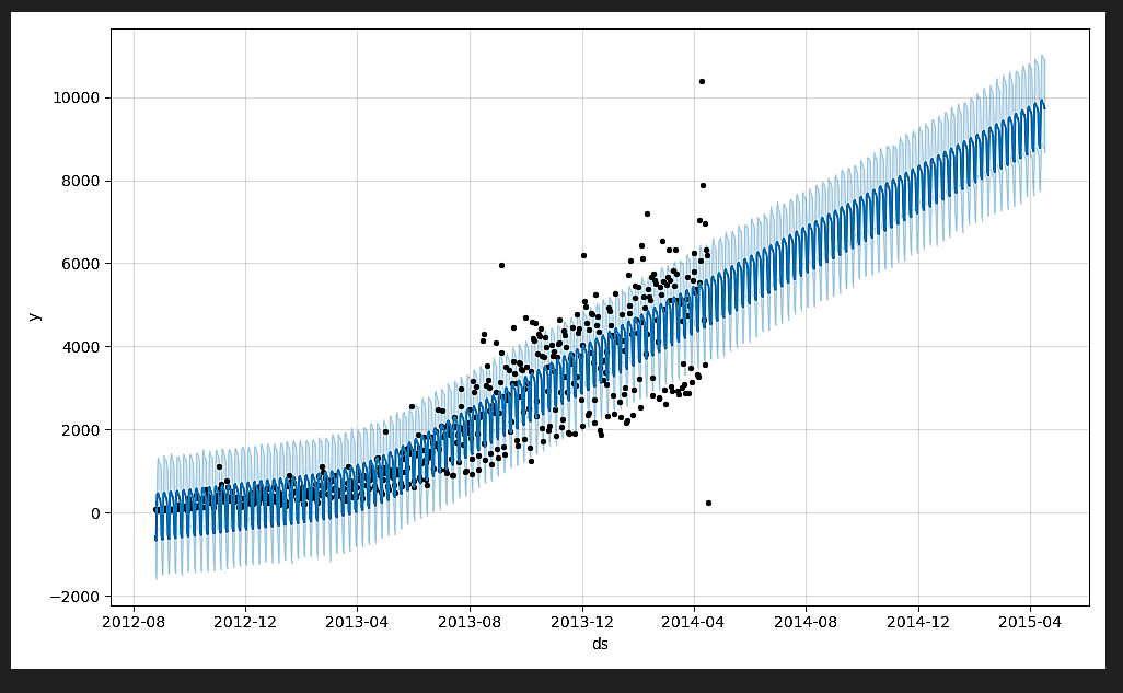
    m.plot(forecast).savefig("train1.png")
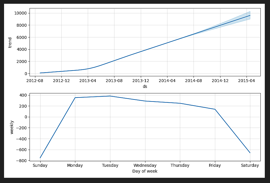
    m.plot_components(forecast).savefig("train2.png")
    # m.plot(forecast).save()
    # print(type(forecast))
    print("Saving file ......")
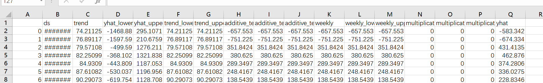
    forecast.to_csv("trainOut.csv")

其中由于m.plot().show() 显示图片会一闪而过 , 所以这里改用savefig将图片保存

forecast为DataFrame, 直接可以保存为csv

其中最后一列为预测值

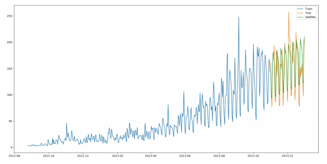
对比预测结果&真实结果:

这里由于python自带的绘图太模糊不好调整

直接将数据提出用excel生成

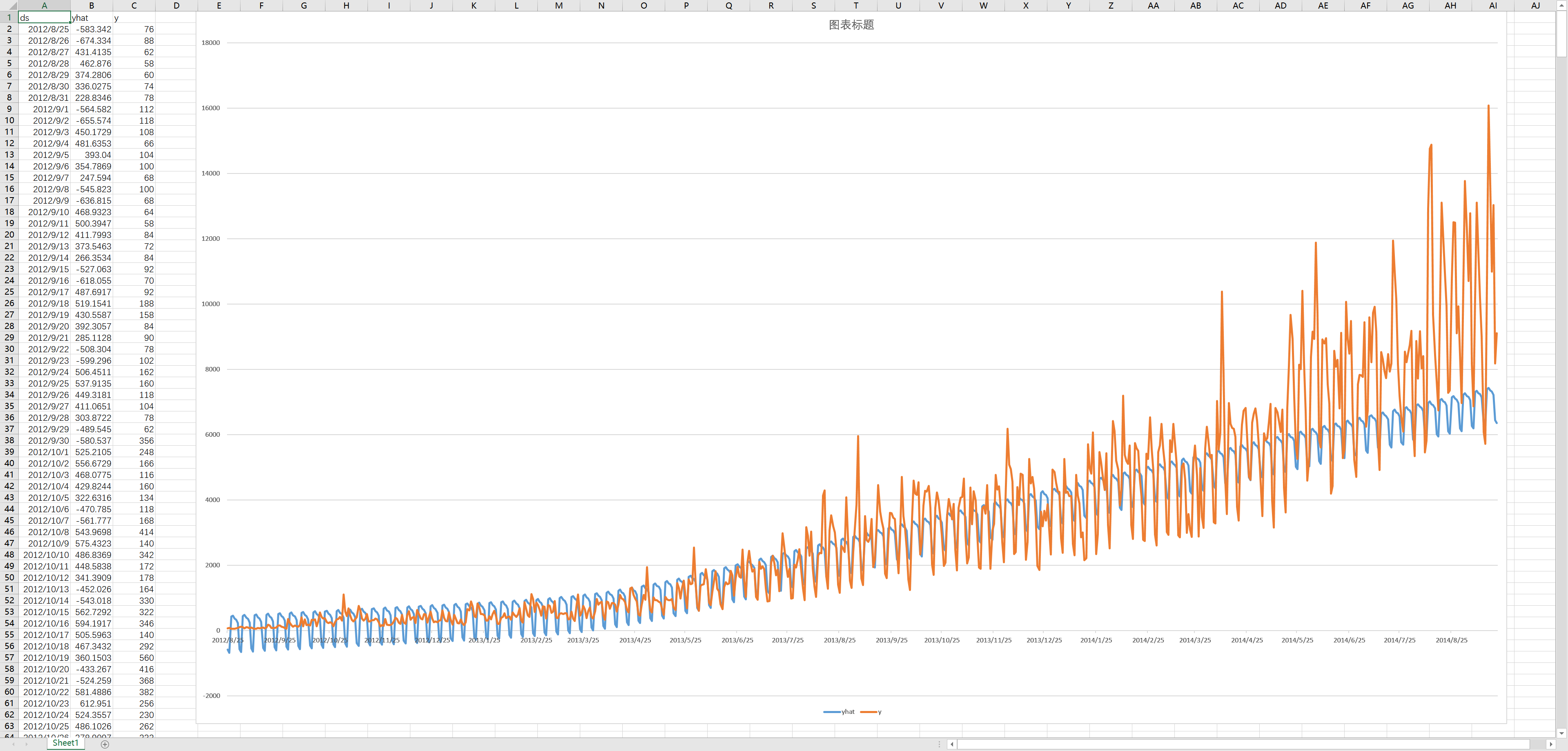
可以看到后头的效果并不是很好

对比于之前的ARIMA模型预测, 可以看出明显的差距:

需要后头的进阶使用