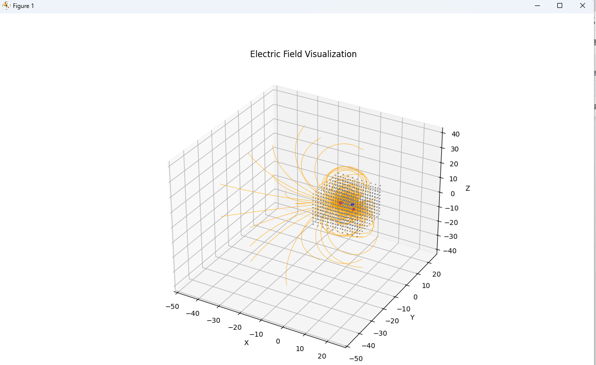
静电场线可视化

静电场线可视化
绘制点电荷或带电体周围的电场线分布，体现电场强度的方向与大小。

import numpy as np
import matplotlib.pyplot as plt
from mpl_toolkits.mplot3d import Axes3D
from matplotlib.patches import Circle
import mpl_toolkits.mplot3d.art3d as art3d


# 定义带电体类
class ChargedObject:
    def __init__(self, position, charge, shape="sphere", size=0.5):
        self.position = np.array(position)
        self.charge = charge
        self.shape = shape
        self.size = size

    def plot(self, ax):
        if self.shape == "sphere":
            u, v = np.mgrid[0:2 * np.pi:20j, 0:np.pi:10j]
            x = self.position[0] + self.size * np.cos(u) * np.sin(v)
            y = self.position[1] + self.size * np.sin(u) * np.sin(v)
            z = self.position[2] + self.size * np.cos(v)
            ax.plot_wireframe(x, y, z, color='r' if self.charge > 0 else 'b')
        elif self.shape == "box":
            # 定义长方体的顶点
            x = [self.position[0] - self.size / 2, self.position[0] + self.size / 2]
            y = [self.position[1] - self.size / 2, self.position[1] + self.size / 2]
            z = [self.position[2] - self.size / 2, self.position[2] + self.size / 2]
            xx, yy = np.meshgrid(x, y)
            ax.plot_wireframe(xx, yy, np.full_like(xx, z[0]), color='r' if self.charge > 0 else 'b')
            ax.plot_wireframe(xx, yy, np.full_like(xx, z[1]), color='r' if self.charge > 0 else 'b')
            xx, zz = np.meshgrid(x, z)
            ax.plot_wireframe(xx, np.full_like(xx, y[0]), zz, color='r' if self.charge > 0 else 'b')
            ax.plot_wireframe(xx, np.full_like(xx, y[1]), zz, color='r' if self.charge > 0 else 'b')
            yy, zz = np.meshgrid(y, z)
            ax.plot_wireframe(np.full_like(yy, x[0]), yy, zz, color='r' if self.charge > 0 else 'b')
            ax.plot_wireframe(np.full_like(yy, x[1]), yy, zz, color='r' if self.charge > 0 else 'b')


# 计算电场强度
def electric_field(position, charged_objects):
    k = 9e9  # 库仑常数
    E = np.array([0.0, 0.0, 0.0])
    for obj in charged_objects:
        r = position - obj.position
        r_mag = np.linalg.norm(r)
        if r_mag > 1e-10:
            E += k * obj.charge * r / r_mag ** 3
    return E


# 生成电场线起始点
def generate_start_points(charged_obj, num_points=20):
    if charged_obj.shape == "sphere":
        u = np.linspace(0, 2 * np.pi, num_points)
        v = np.linspace(0, np.pi, num_points)
        points = []
        for i in range(num_points):
            for j in range(num_points):
                x = charged_obj.position[0] + charged_obj.size * np.cos(u[i]) * np.sin(v[j])
                y = charged_obj.position[1] + charged_obj.size * np.sin(u[i]) * np.sin(v[j])
                z = charged_obj.position[2] + charged_obj.size * np.cos(v[j])
                points.append(np.array([x, y, z]))
        return points
    elif charged_obj.shape == "box":
        x = [charged_obj.position[0] - charged_obj.size / 2, charged_obj.position[0] + charged_obj.size / 2]
        y = [charged_obj.position[1] - charged_obj.size / 2, charged_obj.position[1] + charged_obj.size / 2]
        z = [charged_obj.position[2] - charged_obj.size / 2, charged_obj.position[2] + charged_obj.size / 2]
        points = []
        for xx in x:
            for yy in y:
                points.append(np.array([xx, yy, z[0]]))
                points.append(np.array([xx, yy, z[1]]))
        for xx in x:
            for zz in z:
                points.append(np.array([xx, y[0], zz]))
                points.append(np.array([xx, y[1], zz]))
        for yy in y:
            for zz in z:
                points.append(np.array([x[0], yy, zz]))
                points.append(np.array([x[1], yy, zz]))
        return points


# 追踪电场线
def trace_field_line(start_point, charged_objects, step_size=0.1, max_steps=500):
    line = [start_point]
    current_point = start_point
    for _ in range(max_steps):
        E = electric_field(current_point, charged_objects)
        E_mag = np.linalg.norm(E)
        if E_mag < 1e-3:
            break
        current_point = current_point + step_size * E / E_mag
        line.append(current_point)
    return np.array(line)


# 创建带电体列表
charged_objects = [
    ChargedObject([-3, 0, 0], 5e-6, shape="sphere", size=0.5),
    ChargedObject([2, 1, 0], -8e-6, shape="box", size=0.6),
    ChargedObject([4, -2, 0], 3e-6, shape="sphere", size=0.4)
]

# 创建 3D 图形
fig = plt.figure(figsize=(12, 8))
ax = fig.add_subplot(111, projection='3d')

# 绘制带电体
for obj in charged_objects:
    obj.plot(ax)

# 绘制电场线
for obj in charged_objects:
    if obj.charge > 0:
        start_points = generate_start_points(obj)
        for start_point in start_points:
            field_line = trace_field_line(start_point, charged_objects)
            ax.plot(field_line[:, 0], field_line[:, 1], field_line[:, 2], color='orange', linewidth=0.5)

# 绘制电场向量
x, y, z = np.meshgrid(np.linspace(-10, 10, 10), np.linspace(-10, 10, 10), np.linspace(-10, 10, 10))
Ex = np.zeros_like(x)
Ey = np.zeros_like(y)
Ez = np.zeros_like(z)
for i in range(x.shape[0]):
    for j in range(x.shape[1]):
        for k in range(x.shape[2]):
            position = np.array([x[i, j, k], y[i, j, k], z[i, j, k]])
            E = electric_field(position, charged_objects)
            Ex[i, j, k] = E[0]
            Ey[i, j, k] = E[1]
            Ez[i, j, k] = E[2]

ax.quiver(x, y, z, Ex, Ey, Ez, length=0.5, normalize=True, color='gray')

# 设置坐标轴标签和标题
ax.set_xlabel('X')
ax.set_ylabel('Y')
ax.set_zlabel('Z')
ax.set_title('Electric Field Visualization')

# 显示图形
plt.show()