CS231n作业+代码实践：Assignment1 k-Nearest Neighbor

首先这里给出Assigment1的下载地址：

http://cs231n.stanford.edu/assignments/2016/winter1516_assignment1.zip	

1.下载数据

下载数据： 一旦有了入门代码，就需要下载CIFAR-10数据集。从assignment1目录运行以下命令：

cd cs231n/datasets
./get_datasets.sh

2.python2和python3的问题

可能因为视频间隔时间比较久，原代码采用的python2的格式，可能会出现以下错误：

   print 'loading training data for synset %d / %d' % (i + 1, len(wnids))
                                                   ^
SyntaxError: invalid syntax

这个时候我们就要找到CS231n文件夹下的data_utils.py的文件，修改成python3的格式（直接复制即可）

from __future__ import print_function

from six.moves import cPickle as pickle
import numpy as np
import os
#from scipy.misc import imread 把这一行注释掉
from imageio import imread #换成这一行
import platform

def load_pickle(f):
    version = platform.python_version_tuple()
    if version[0] == '2':
        return  pickle.load(f)
    elif version[0] == '3':
        return  pickle.load(f, encoding='latin1')
    raise ValueError("invalid python version: {}".format(version))

def load_CIFAR_batch(filename):
  """ load single batch of cifar """
  with open(filename, 'rb') as f:
    datadict = load_pickle(f)
    X = datadict['data']
    Y = datadict['labels']
    X = X.reshape(10000, 3, 32, 32).transpose(0,2,3,1).astype("float")
    Y = np.array(Y)
    return X, Y

def load_CIFAR10(ROOT):
  """ load all of cifar """
  xs = []
  ys = []
  for b in range(1,6):
    f = os.path.join(ROOT, 'data_batch_%d' % (b, ))
    X, Y = load_CIFAR_batch(f)
    xs.append(X)
    ys.append(Y)    
  Xtr = np.concatenate(xs)
  Ytr = np.concatenate(ys)
  del X, Y
  Xte, Yte = load_CIFAR_batch(os.path.join(ROOT, 'test_batch'))
  return Xtr, Ytr, Xte, Yte


def get_CIFAR10_data(num_training=49000, num_validation=1000, num_test=1000,
                     subtract_mean=True):
    """
    Load the CIFAR-10 dataset from disk and perform preprocessing to prepare
    it for classifiers. These are the same steps as we used for the SVM, but
    condensed to a single function.
    """
    # Load the raw CIFAR-10 data
    cifar10_dir = 'cs231n/datasets/cifar-10-batches-py'
    X_train, y_train, X_test, y_test = load_CIFAR10(cifar10_dir)
        
    # Subsample the data
    mask = list(range(num_training, num_training + num_validation))
    X_val = X_train[mask]
    y_val = y_train[mask]
    mask = list(range(num_training))
    X_train = X_train[mask]
    y_train = y_train[mask]
    mask = list(range(num_test))
    X_test = X_test[mask]
    y_test = y_test[mask]

    # Normalize the data: subtract the mean image
    if subtract_mean:
      mean_image = np.mean(X_train, axis=0)
      X_train -= mean_image
      X_val -= mean_image
      X_test -= mean_image
    
    # Transpose so that channels come first
    X_train = X_train.transpose(0, 3, 1, 2).copy()
    X_val = X_val.transpose(0, 3, 1, 2).copy()
    X_test = X_test.transpose(0, 3, 1, 2).copy()

    # Package data into a dictionary
    return {
      'X_train': X_train, 'y_train': y_train,
      'X_val': X_val, 'y_val': y_val,
      'X_test': X_test, 'y_test': y_test,
    }
    

def load_tiny_imagenet(path, dtype=np.float32, subtract_mean=True):
  """
  Load TinyImageNet. Each of TinyImageNet-100-A, TinyImageNet-100-B, and
  TinyImageNet-200 have the same directory structure, so this can be used
  to load any of them.

  Inputs:
  - path: String giving path to the directory to load.
  - dtype: numpy datatype used to load the data.
  - subtract_mean: Whether to subtract the mean training image.

  Returns: A dictionary with the following entries:
  - class_names: A list where class_names[i] is a list of strings giving the
    WordNet names for class i in the loaded dataset.
  - X_train: (N_tr, 3, 64, 64) array of training images
  - y_train: (N_tr,) array of training labels
  - X_val: (N_val, 3, 64, 64) array of validation images
  - y_val: (N_val,) array of validation labels
  - X_test: (N_test, 3, 64, 64) array of testing images.
  - y_test: (N_test,) array of test labels; if test labels are not available
    (such as in student code) then y_test will be None.
  - mean_image: (3, 64, 64) array giving mean training image
  """
  # First load wnids
  with open(os.path.join(path, 'wnids.txt'), 'r') as f:
    wnids = [x.strip() for x in f]

  # Map wnids to integer labels
  wnid_to_label = {wnid: i for i, wnid in enumerate(wnids)}

  # Use words.txt to get names for each class
  with open(os.path.join(path, 'words.txt'), 'r') as f:
    wnid_to_words = dict(line.split('\t') for line in f)
    for wnid, words in wnid_to_words.iteritems():
      wnid_to_words[wnid] = [w.strip() for w in words.split(',')]
  class_names = [wnid_to_words[wnid] for wnid in wnids]

  # Next load training data.
  X_train = []
  y_train = []
  for i, wnid in enumerate(wnids):
    if (i + 1) % 20 == 0:
      print('loading training data for synset %d / %d' % (i + 1, len(wnids)))
    # To figure out the filenames we need to open the boxes file
    boxes_file = os.path.join(path, 'train', wnid, '%s_boxes.txt' % wnid)
    with open(boxes_file, 'r') as f:
      filenames = [x.split('\t')[0] for x in f]
    num_images = len(filenames)
    
    X_train_block = np.zeros((num_images, 3, 64, 64), dtype=dtype)
    y_train_block = wnid_to_label[wnid] * np.ones(num_images, dtype=np.int64)
    for j, img_file in enumerate(filenames):
      img_file = os.path.join(path, 'train', wnid, 'images', img_file)
      img = imread(img_file)
      if img.ndim == 2:
        ## grayscale file
        img.shape = (64, 64, 1)
      X_train_block[j] = img.transpose(2, 0, 1)
    X_train.append(X_train_block)
    y_train.append(y_train_block)
      
  # We need to concatenate all training data
  X_train = np.concatenate(X_train, axis=0)
  y_train = np.concatenate(y_train, axis=0)
  
  # Next load validation data
  with open(os.path.join(path, 'val', 'val_annotations.txt'), 'r') as f:
    img_files = []
    val_wnids = []
    for line in f:
      img_file, wnid = line.split('\t')[:2]
      img_files.append(img_file)
      val_wnids.append(wnid)
    num_val = len(img_files)
    y_val = np.array([wnid_to_label[wnid] for wnid in val_wnids])
    X_val = np.zeros((num_val, 3, 64, 64), dtype=dtype)
    for i, img_file in enumerate(img_files):
      img_file = os.path.join(path, 'val', 'images', img_file)
      img = imread(img_file)
      if img.ndim == 2:
        img.shape = (64, 64, 1)
      X_val[i] = img.transpose(2, 0, 1)

  # Next load test images
  # Students won't have test labels, so we need to iterate over files in the
  # images directory.
  img_files = os.listdir(os.path.join(path, 'test', 'images'))
  X_test = np.zeros((len(img_files), 3, 64, 64), dtype=dtype)
  for i, img_file in enumerate(img_files):
    img_file = os.path.join(path, 'test', 'images', img_file)
    img = imread(img_file)
    if img.ndim == 2:
      img.shape = (64, 64, 1)
    X_test[i] = img.transpose(2, 0, 1)

  y_test = None
  y_test_file = os.path.join(path, 'test', 'test_annotations.txt')
  if os.path.isfile(y_test_file):
    with open(y_test_file, 'r') as f:
      img_file_to_wnid = {}
      for line in f:
        line = line.split('\t')
        img_file_to_wnid[line[0]] = line[1]
    y_test = [wnid_to_label[img_file_to_wnid[img_file]] for img_file in img_files]
    y_test = np.array(y_test)
  
  mean_image = X_train.mean(axis=0)
  if subtract_mean:
    X_train -= mean_image[None]
    X_val -= mean_image[None]
    X_test -= mean_image[None]

  return {
    'class_names': class_names,
    'X_train': X_train,
    'y_train': y_train,
    'X_val': X_val,
    'y_val': y_val,
    'X_test': X_test,
    'y_test': y_test,
    'class_names': class_names,
    'mean_image': mean_image,
  }


def load_models(models_dir):
  """
  Load saved models from disk. This will attempt to unpickle all files in a
  directory; any files that give errors on unpickling (such as README.txt) will
  be skipped.

  Inputs:
  - models_dir: String giving the path to a directory containing model files.
    Each model file is a pickled dictionary with a 'model' field.

  Returns:
  A dictionary mapping model file names to models.
  """
  models = {}
  for model_file in os.listdir(models_dir):
    with open(os.path.join(models_dir, model_file), 'rb') as f:
      try:
        models[model_file] = load_pickle(f)['model']
      except pickle.UnpicklingError:
        continue
  return models

3.导入数据集

# Run some setup code for this notebook.
from __future__ import print_function
import random
import numpy as np
from cs231n.data_utils import load_CIFAR10
import matplotlib.pyplot as plt


# This is a bit of magic to make matplotlib figures appear inline in the notebook
# rather than in a new window.
%matplotlib inline
plt.rcParams['figure.figsize'] = (10.0, 8.0) # set default size of plots
plt.rcParams['image.interpolation'] = 'nearest'
plt.rcParams['image.cmap'] = 'gray'

# Some more magic so that the notebook will reload external python modules;
# see http://stackoverflow.com/questions/1907993/autoreload-of-modules-in-ipython
%load_ext autoreload 
%autoreload 2

其中值得注意的是%load_ext autoreload %autoreload 2，在作业中讲到，这段代码表示在外面修改文件时，notebook会自动更新，不需要每次再重新执行代码。

在本次作业中，这两行十分关键，因为我们有需要修改linear_classifier.py的任务。运行后出现：

The autoreload extension is already loaded. To reload it, use:
  %reload_ext autoreload

维度检测十分重要，对于检验bug很有用，在深度学习里很多错误都是来自于矩阵的维度有误。一般用reshape来展示矩阵的维度。

# Load the raw CIFAR-10 data.
cifar10_dir = 'cs231n/datasets/cifar-10-batches-py'

# Cleaning up variables to prevent loading data multiple times (which may cause memory issue)
try:
   del X_train, y_train
   del X_test, y_test
   print('Clear previously loaded data.')
except:
   pass

X_train, y_train, X_test, y_test = load_CIFAR10(cifar10_dir)

# As a sanity check, we print out the size of the training and test data.
print('Training data shape: ', X_train.shape)
print('Training labels shape: ', y_train.shape)
print('Test data shape: ', X_test.shape)
print('Test labels shape: ', y_test.shape)

Training data shape:  (50000, 32, 32, 3)
Training labels shape:  (50000,)
Test data shape:  (10000, 32, 32, 3)
Test labels shape:  (10000,)

在做深度学习深度学习的时候，我们通常会显示我们的dataset,常常会用到matplotlib函数里的pyplot库。这里选择展示样例的图片为10张，然后用subplot函数去组合排列好。（这个方法比较好，可以学习！）

# Visualize some examples from the dataset.#显示图片
# We show a few examples of training images from each class.
classes = ['plane', 'car', 'bird', 'cat', 'deer', 'dog', 'frog', 'horse', 'ship', 'truck']
num_classes = len(classes) #7
samples_per_class = 10
for y, cls in enumerate(classes):
    idxs = np.flatnonzero(y_train == y)#返回第i类图片编号
    idxs = np.random.choice(idxs, samples_per_class, replace=False)#随机选一些图片show
    for i, idx in enumerate(idxs):
        plt_idx = i * num_classes + y + 1
        plt.subplot(samples_per_class, num_classes, plt_idx)
        plt.imshow(X_train[idx].astype('uint8'))
        plt.axis('off')
        if i == 0:
            plt.title(cls)
plt.show()

输出得到这样的图片格式：

4.预实验

因为原照片集比较大，所以我们选择5000张照片作为训练样本，500个测试样本来先进行预实验。

# Subsample the data for more efficient code execution in this exercise
num_training = 5000
mask = list(range(num_training)) #生成0-4999的序列
X_train = X_train[mask] #输入前5000个样本的信息
y_train = y_train[mask]
num_test = 500 #输入前500个样本的信息
mask = list(range(num_test))
X_test = X_test[mask]
y_test = y_test[mask]

这里值得注意的是X_train作为一个数组，他的索引可以为一个列表，用来表示前5000张图片。

# Reshape the image data into rows
X_train = np.reshape(X_train, (X_train.shape[0], -1))
X_test = np.reshape(X_test, (X_test.shape[0], -1))
print(X_train.shape, X_test.shape)

因为图片有X_traiin有四个维度，我们要把后三个维度给拉平，得到（5000,3072）的数组

(5000, 3072) (500, 3072)

这里如果看一下k_nearest_neighbor.py文件，会发现里面创建了一个KNearestNeighbor类，下面将进行对类操作。

from cs231n.classifiers import KNearestNeighbor
# Create a kNN classifier instance. 
# Remember that training a kNN classifier is a noop空操作: 
# the Classifier simply remembers the data and does no further processing 
classifier = KNearestNeighbor()
classifier.train(X_train, y_train)

那么下面就是要打开k_nearest_neighbor.py文件去完成里面的方法了！

  def train(self, X, y):
    """
    Train the classifier. For k-nearest neighbors this is just 
    memorizing the training data.

    Inputs:
    - X: A numpy array of shape (num_train, D) containing the training data
      consisting of num_train samples each of dimension D.
    - y: A numpy array of shape (N,) containing the training labels, where
         y[i] is the label for X[i].
    """
    self.X_train = X
    self.y_train = y

这是说是训练X,y的代码，其实只是保存了X，y作为类里的属性，方便后面进行predict，这在之后的NN网络里也是这样使用的。下面才开始正式训练了。

 def compute_distances_two_loops(self, X):
    """
    Compute the distance between each test point in X and each training point
    in self.X_train using a nested loop over both the training data and the 
    test data.

    Inputs:
    - X: A numpy array of shape (num_test, D) containing test data.

    Returns:
    - dists: A numpy array of shape (num_test, num_train) where dists[i, j]
      is the Euclidean distance between the ith test point and the jth training
      point.
    """
    num_test = X.shape[0] #测试样本
    num_train = self.X_train.shape[0] #classifer 里面的训练样本
    dists = np.zeros((num_test, num_train)) #初始化
    for i in range(num_test):
      for j in range(num_train):
        #####################################################################
        # TODO:                                                             #
        # Compute the l2 distance between the ith test point and the jth    #
        # training point, and store the result in dists[i, j]. You should   #
        # not use a loop over dimension.                                    #
        #####################################################################
        dists[i,j] = np.linalg.norm(X[i,:]-self.X_train[j,:], ord=2)
        #####################################################################
        #                       END OF YOUR CODE                            #
        #####################################################################
    return dists

这个代码是用两层循环loop来写的，分别把训练集和测试集各遍历了一遍，这样的速度较慢，时间复杂度较高（后面会测试，一般我们都是用vector化去表示）,np.linalg.norm(X[i,:]self.X_train[j,:], ord=2)表示使用了二范数去计算distance。

def compute_distances_one_loop(self, X):
    """
    Compute the distance between each test point in X and each training point
    in self.X_train using a single loop over the test data.

    Input / Output: Same as compute_distances_two_loops
    """
    num_test = X.shape[0]
    num_train = self.X_train.shape[0]
    dists = np.zeros((num_test, num_train))
    for i in range(num_test):
      #######################################################################
      # TODO:                                                               #
      # Compute the l2 distance between the ith test point and all training #
      # points, and store the result in dists[i, :].                        #
      #######################################################################
      dists[i] = np.linalg.norm(X[i] - self.X_train, ord=2，axis=1)
      #######################################################################
      #                         END OF YOUR CODE                            #
      #######################################################################
    return dists

相对于上面的代码来说，这次一层循环更简单了，思考方式来源于，我们其实可以一行一行去遍历，利用python中广播的特性，可以不需要遍历训练集。这个速度更快一点。
在这里我详细写一下，X[i]维度是（1,784），self.X_train维度是（500,784），根据广播原理，相减是（500,784）。axis=1代表对列方向求范数，因此再对列方向求和，则压缩成一行维度是（1,784）。对i进行遍历，便形成了（5000,500）维度的dist矩阵。（这里要比上面一次循环的要难一点）

def compute_distances_no_loops(self, X):
    """
    Compute the distance between each test point in X and each training point
    in self.X_train using no explicit loops.

    Input / Output: Same as compute_distances_two_loops
    """
    num_test = X.shape[0]
    num_train = self.X_train.shape[0]
    dists = np.zeros((num_test, num_train)) 
    #########################################################################
    # TODO:                                                                 #
    # Compute the l2 distance between all test points and all training      #
    # points without using any explicit loops, and store the result in      #
    # dists.                                                                #
    #                                                                       #
    # You should implement this function using only basic array operations; #
    # in particular you should not use functions from scipy.                #
    #                                                                       #
    # HINT: Try to formulate the l2 distance using matrix multiplication 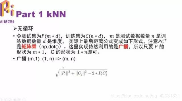   #![在这里插入图片描述](https://img-blog.csdnimg.cn/20200416192826733.jpeg?x-oss-process=image/watermark,type_ZmFuZ3poZW5naGVpdGk,shadow_10,text_aHR0cHM6Ly9ibG9nLmNzZG4ubmV0L3FxXzQyOTMxODMx,size_16,color_FFFFFF,t_70)
    #       and two broadcast sums.                                         #
    #########################################################################
    test_sum = np.sum(np.square(X), axis=1)  # 500*3072 - 500*1 以500,形式表示
    train_sum = np.sum(np.square(self.X_train), axis=1)  # 5000*3072 - 5000*1 以5000,形式表示
    dianji = np.dot(X, self.X_train.T)  # 点积(转置)500*5000
    dists = np.sqrt(-2 * dianji + test_sum.reshape(-1,1) + train_sum.reshape(1,-1))  # 平方展开，广播
    #########################################################################
    #                         END OF YOUR CODE                              #
    #########################################################################
    return dists

这个是无循环，在提示里讲到了要用vector去做运算，这个一开始我没有想到，后来看到了一篇帖子豁然开朗。需要一点数学推导，我先把他放上：

应该算是用了一个完全平方公式，但是是矩阵的计算，所以我们要检查一下维度，训练集集对自己做内积然后按行求和得到（5000，1）,同理测试集按行求和得到（500,1），中间两项乘积（5000,500），我们发现三项可以用广播加减，得到（5000,500）维度。（这边之前看到一个很好看的数学推导，现在没找到，后面补上）
我们来实验一下：

# Open cs231n/classifiers/k_nearest_neighbor.py and implement
# compute_distances_two_loops.

# Test your implementation:
dists = classifier.compute_distances_no_loops(X_test)
print(dists.shape)
# We can visualize the distance matrix: each row is a single test example and
# its distances to training examples
plt.imshow(dists, interpolation='none')
plt.show()

• 白色距离远，黑色距离近，越黑越近

下面写一下predict函数：

def predict_labels(self, dists, k):
    """
    Given a matrix of distances between test points and training points,
    predict a label for each test point.

    Inputs:
    - dists: A numpy array of shape (num_test, num_train) where dists[i, j]
      gives the distance betwen the ith test point and the jth training point.

    Returns:
    - y: A numpy array of shape (num_test,) containing predicted labels for the
      test data, where y[i] is the predicted label for the test point X[i].  
    """
    num_test = dists.shape[0] #输入测试集的数量
    y_pred = np.zeros(num_test) #测试的结果输出，维度与输入一致
    for i in range(num_test):
      # A list of length k storing the labels of the k nearest neighbors to
      # the ith test point.
      closest_y = []
      #########################################################################
      # TODO:                                                                 #
      # Use the distance matrix to find the k nearest neighbors of the ith    #
      # testing point, and use self.y_train to find the labels of these       #
      # neighbors. Store these labels in closest_y.                           #
      # Hint: Look up the function numpy.argsort.                             #
      #########################################################################
      label = np.argsort(dists[i,:],axis=0)
      closest_y = self.y_train[label[:k]]
      #########################################################################
      # TODO:                                                                 #
      # Now that you have found the labels of the k nearest neighbors, you    #
      # need to find the most common label in the list closest_y of labels.   #
      # Store this label in y_pred[i]. Break ties by choosing the smaller     #
      # label.                                                                #
      #########################################################################
      y_pred[i] = np.argmax(np.bincount(closest_y))
      #########################################################################
      #                           END OF YOUR CODE                            # 
      #########################################################################

    return y_pred

其中 np.argsort用来对数组进行排序，这里axis=0表示按行排序，输出一个从大到小排列的数组的索引（注意这里是索引）， np.argmax(np.bincount(closest_y))这里用来求出现次数最多的值，是个常用的组合函数。

然后开始预测

# Now implement the function predict_labels and run the code below:
# We use k = 1 (which is Nearest Neighbor).
y_test_pred = classifier.predict_labels(dists, k=1)

# Compute and print the fraction of correctly predicted examples
num_correct = np.sum(y_test_pred == y_test)
accuracy = float(num_correct) / num_test
print('Got %d / %d correct => accuracy: %f' % (num_correct, num_test, accuracy))

Got 137 / 500 correct => accuracy: 0.274000

y_test_pred = classifier.predict_labels(dists, k=5)
num_correct = np.sum(y_test_pred == y_test)
accuracy = float(num_correct) / num_test
print('Got %d / %d correct => accuracy: %f' % (num_correct, num_test, accuracy))

Got 139 / 500 correct => accuracy: 0.278000

5.比较时间复杂度和准确率

# Now lets speed up distance matrix computation by using partial vectorization
# with one loop. Implement the function compute_distances_one_loop and run the
# code below:
dists_one = classifier.compute_distances_one_loop(X_test)

# To ensure that our vectorized implementation is correct, we make sure that it
# agrees with the naive implementation. There are many ways to decide whether
# two matrices are similar; one of the simplest is the Frobenius norm. In case
# you haven't seen it before, the Frobenius norm of two matrices is the square
# root of the squared sum of differences of all elements; in other words, reshape
# the matrices into vectors and compute the Euclidean distance between them.
difference = np.linalg.norm(dists - dists_one, ord='fro')
print('Difference was: %f' % (difference, ))
if difference < 0.001:
    print('Good! The distance matrices are the same')
else:
    print('Uh-oh! The distance matrices are different')

Difference was: 0.000000
Good! The distance matrices are the same

# Now implement the fully vectorized version inside compute_distances_no_loops
# and run the code
dists_two = classifier.compute_distances_no_loops(X_test)

# check that the distance matrix agrees with the one we computed before:
difference = np.linalg.norm(dists - dists_two, ord='fro')
print('Difference was: %f' % (difference, ))
if difference < 0.001:
    print('Good! The distance matrices are the same')
else:
    print('Uh-oh! The distance matrices are different')

Difference was: 0.000000
Good! The distance matrices are the same

# Let's compare how fast the implementations are
def time_function(f, *args):
    """
    Call a function f with args and return the time (in seconds) that it took to execute.
    """
    import time
    tic = time.time()
    f(*args)
    toc = time.time()
    return toc - tic

two_loop_time = time_function(classifier.compute_distances_two_loops, X_test)
print('Two loop version took %f seconds' % two_loop_time)

one_loop_time = time_function(classifier.compute_distances_one_loop, X_test)
print('One loop version took %f seconds' % one_loop_time)

no_loop_time = time_function(classifier.compute_distances_no_loops, X_test)
print('No loop version took %f seconds' % no_loop_time)

# you should see significantly faster performance with the fully vectorized implementation

Two loop version took 30.444194 seconds
One loop version took 44.425471 seconds
No loop version took 0.213420 seconds

6.交叉验证集

这一段代码比较长，我们分解来看

num_folds = 5
k_choices = [1, 3, 5, 8, 10, 12, 15, 20, 50, 100]

X_train_folds = []
y_train_folds = []

这里告诉我们，交叉验证集选择5份（其中4份做训练，1份做验证），同时，选择不同k个样本进行投票。

################################################################################
# TODO:                                                                        #
# Split up the training data into folds. After splitting, X_train_folds and    #
# y_train_folds should each be lists of length num_folds, where                #
# y_train_folds[i] is the label vector for the points in X_train_folds[i].     #
# Hint: Look up the numpy array_split function.                                #
################################################################################
X_train_folds = np.array_split(X_train,num_folds)
y_train_folds = np.array_split(y_train,num_folds)

###############################################################################
#                                 END OF YOUR CODE                             #
################################################################################

提示已经告诉我们，用np.array_split()函数可以把数组分组。用这个函数把上面分成5组。

# A dictionary holding the accuracies for different values of k that we find
# when running cross-validation. After running cross-validation,
# k_to_accuracies[k] should be a list of length num_folds giving the different
# accuracy values that we found when using that value of k.
k_to_accuracies = {}
for k in k_choices:
    k_to_accuracies.setdefault(k,[]) #添加空值 字典加key ，建立空字典
################################################################################
# TODO:                                                                        #
# Perform k-fold cross validation to find the best value of k. For each        #
# possible value of k, run the k-nearest-neighbor algorithm num_folds times,   #
# where in each case you use all but one of the folds as training data and the #
# last fold as a validation set. Store the accuracies for all fold and all     #
# values of k in the k_to_accuracies dictionary.                               #
################################################################################
for k in k_choices:  #
    print(k)
    classifier = KNearestNeighbor()
    for i in range(num_folds):  #5次
        x_val_train = np.vstack(X_train_folds[0:i]+X_train_folds[i+1:])  #交叉验证
        y_val_train = np.vstack(y_train_folds[0:i]+y_train_folds[i+1:])
        y_val_train = y_val_train.reshape(4000)
        #rint(y_train_folds[i])
        classifier.train(x_val_train, y_val_train)
        dists = classifier.compute_distances_no_loops(X_train_folds[i])
        y_test_pred = classifier.predict_labels(dists, k=k)
        num_correct = np.sum(y_test_pred == y_train_folds[i])
        accuracy = float(num_correct) / len(y_test_pred)
        #以上几步都是照抄前面的预测
        k_to_accuracies[k] = k_to_accuracies[k]+[accuracy]  #加到dict多个值
        print(k_to_accuracies)
################################################################################
#                                 END OF YOUR CODE                             #
################################################################################

# Print out the computed accuracies
for k in sorted(k_to_accuracies):
    for accuracy in k_to_accuracies[k]:
        print('k = %d, accuracy = %f' % (k, accuracy))

这里有两层循环，第一层我们循环不同的k类，接着我们用交叉验证法做出5个不同的验证集的结果，最后把它传到 k_to_accuracies中，其中训练的部分可以用我们之前的函数（这里建议用no_loop)。要注意的是这边k_to_accuracies每个Key对应的value是一个列表，其中有五个数。为了直观，我这边加了一个print.(太长了，我这边摘一点结果）

1
{1: [0.263], 3: [], 5: [], 8: [], 10: [], 12: [], 15: [], 20: [], 50: [], 100: []}
{1: [0.263, 0.257], 3: [], 5: [], 8: [], 10: [], 12: [], 15: [], 20: [], 50: [], 100: []}
{1: [0.263, 0.257, 0.264], 3: [], 5: [], 8: [], 10: [], 12: [], 15: [], 20: [], 50: [], 100: []}
{1: [0.263, 0.257, 0.264, 0.278], 3: [], 5: [], 8: [], 10: [], 12: [], 15: [], 20: [], 50: [], 100: []}
{1: [0.263, 0.257, 0.264, 0.278, 0.266], 3: [], 5: [], 8: [], 10: [], 12: [], 15: [], 20: [], 50: [], 100: []}
3
{1: [0.263, 0.257, 0.264, 0.278, 0.266], 3: [0.239], 5: [], 8: [], 10: [], 12: [], 15: [], 20: [], 50: [], 100: []}
{1: [0.263, 0.257, 0.264, 0.278, 0.266], 3: [0.239, 0.249], 5: [], 8: [], 10: [], 12: [], 15: [], 20: [], 50: [], 100: []}
{1: [0.263, 0.257, 0.264, 0.278, 0.266], 3: [0.239, 0.249, 0.24], 5: [], 8: [], 10: [], 12: [], 15: [], 20: [], 50: [], 100: []}
{1: [0.263, 0.257, 0.264, 0.278, 0.266], 3: [0.239, 0.249, 0.24, 0.266], 5: [], 8: [], 10: [], 12: [], 15: [], 20: [], 50: [], 100: []}
{1: [0.263, 0.257, 0.264, 0.278, 0.266], 3: [0.239, 0.249, 0.24, 0.266, 0.254], 5: [], 8: [], 10: [], 12: [], 15: [], 20: [], 50: [], 100: []}


k = 1, accuracy = 0.263000
k = 1, accuracy = 0.257000
k = 1, accuracy = 0.264000
k = 1, accuracy = 0.278000
k = 1, accuracy = 0.266000
k = 3, accuracy = 0.239000
k = 3, accuracy = 0.249000
k = 3, accuracy = 0.240000
k = 3, accuracy = 0.266000
k = 3, accuracy = 0.254000
k = 5, accuracy = 0.248000
k = 5, accuracy = 0.266000
k = 5, accuracy = 0.280000

最后我们就可以用图像表示，当看到图的时候，内心还是有一点爽感的！

# plot the raw observations
for k in k_choices:
    accuracies = k_to_accuracies[k]
    plt.scatter([k] * len(accuracies), accuracies)

# plot the trend line with error bars that correspond to standard deviation
accuracies_mean = np.array([np.mean(v) for k,v in sorted(k_to_accuracies.items())])
accuracies_std = np.array([np.std(v) for k,v in sorted(k_to_accuracies.items())])
plt.errorbar(k_choices, accuracies_mean, yerr=accuracies_std)
plt.title('Cross-validation on k')
plt.xlabel('k')
plt.ylabel('Cross-validation accuracy')
plt.show()

这边因为有5个输出，所以我们画图的时候用errorbar函数来画，只需要输入横坐标，纵坐标均值还有方差就可以了。

最后一步我们用最好的k去计算准确率：

# Based on the cross-validation results above, choose the best value for k,   
# retrain the classifier using all the training data, and test it on the test
# data. You should be able to get above 28% accuracy on the test data.
best_k = 1

classifier = KNearestNeighbor()
classifier.train(X_train, y_train)
y_test_pred = classifier.predict(X_test, k=best_k)

# Compute and display the accuracy
num_correct = np.sum(y_test_pred == y_test)
accuracy = float(num_correct) / num_test
print('Got %d / %d correct => accuracy: %f' % (num_correct, num_test, accuracy))

Got 137 / 500 correct => accuracy: 0.274000

可以发现准确率还不是很高，所以我们还要学习后面的方法鸭！第一篇博客，有很多漏洞，希望大家批评指正！