BIOS14:Statistic Exercise 3

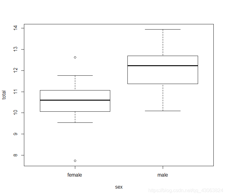
a) Is there a difference between the sexes with respect to total tree-felling? (3p)

Firstly, I imported the data and checked. Then I calculated the total tree-felling data. According to the question, plot the data with boxplot. And I made the assumption that there is no difference between sexes with respect to total tree-felling. And I would use two-sample test to test this.

elefell = read.csv('elefell.csv')
elefell$total = elefell$t1+elefell$t2+elefell$t3+elefell$t4
boxplot(total~sex, data = elefell)

Test the assumptions of a two-sample t-test:

# Normality of data within each group
elemale = subset(elefell, elefell$sex == 'male')
elefemale = subset(elefell, elefell$sex == 'female')
x = elemale$total
h = hist(x)
xfit = seq(min(x, na.rm=TRUE),max(x, na.rm=TRUE),length=100)
yfit = dnorm(xfit,mean=mean(x, na.rm=TRUE),sd=sd(x, na.rm=TRUE))
yfit = yfit*max(h$counts)/max(yfit)
hist(elemale$total, col="red")
lines(xfit, yfit, lwd=2)

> shapiro.test(elemale$total)

	Shapiro-Wilk normality test

data:  elemale$total
W = 0.98058, p-value = 0.9414

> x = elemale$total
> y = pnorm(summary(x), mean =mean(x, na.rm=TRUE), sd =sd(x, na.rm=TRUE))
> ks.test(x, y)

	Two-sample Kolmogorov-Smirnov test

data:  x and y
D = 1, p-value = 8.687e-06
alternative hypothesis: two-sided

> qqnorm(elemale$total)
> qqline(elemale$total)

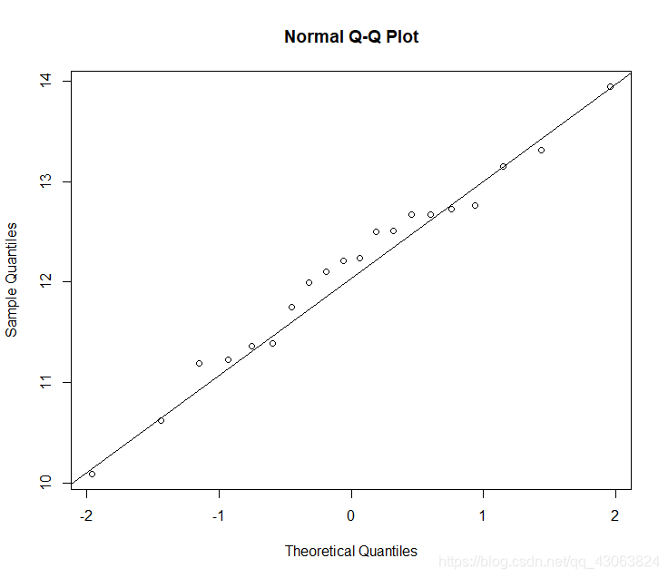
Shapiro-Wilks test is not significant, so we can accept the data as being normal.

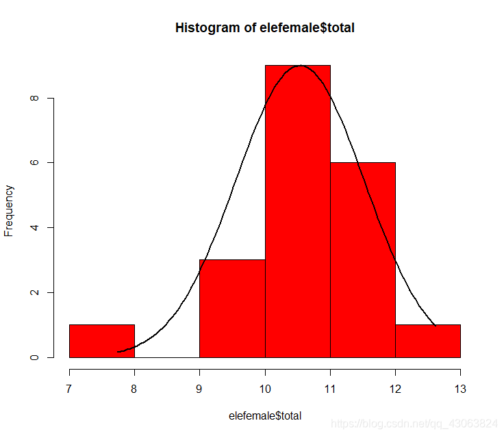
x = elefemale$total
h = hist(x)
xfit = seq(min(x, na.rm=TRUE),max(x, na.rm=TRUE),length=100)
yfit = dnorm(xfit,mean=mean(x, na.rm=TRUE),sd=sd(x, na.rm=TRUE))
yfit = yfit*max(h$counts)/max(yfit)
hist(elefemale$total, col="red")
lines(xfit, yfit, lwd=2)

> shapiro.test(elefemale$total)

	Shapiro-Wilk normality test

data:  elefemale$total
W = 0.93097, p-value = 0.1612

> x = elefemale$total
> y = pnorm(summary(x), mean =mean(x, na.rm=TRUE), sd =sd(x, na.rm=TRUE))
> ks.test(x, y)

	Two-sample Kolmogorov-Smirnov test

data:  x and y
D = 1, p-value = 2.252e-06
alternative hypothesis: two-sided

> qqnorm(elefemale$total)
> qqline(elefemale$total)

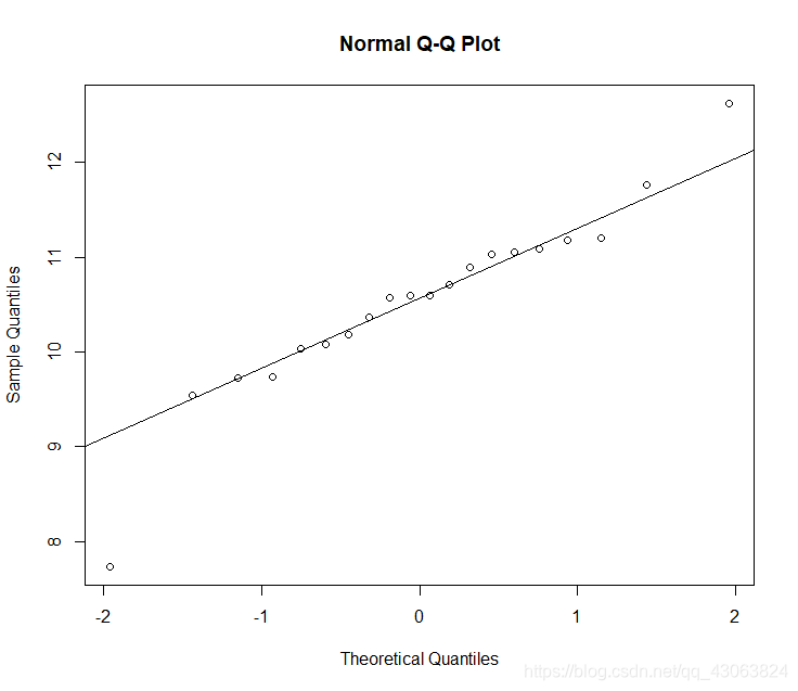
qq-plot looks so-so, Shapiro-Wilks test is not significant, normality is fulfilled.

# Homogeneity of variances
> leveneTest(total~sex, data = elefell)
Levene's Test for Homogeneity of Variance (center = median)
      Df F value Pr(>F)
group  1  0.0596 0.8085
      38             

not significantly different.

#Carry out two-sample t-test
> t.test(total~sex, data = elefell, var.equal=TRUE)

	Two Sample t-test

data:  total by sex
t = -5.2142, df = 38, p-value = 6.787e-06
alternative hypothesis: true difference in means is not equal to 0
95 percent confidence interval:
 -2.2025661 -0.9705997
sample estimates:
mean in group female   mean in group male 
            10.53565             12.12224 

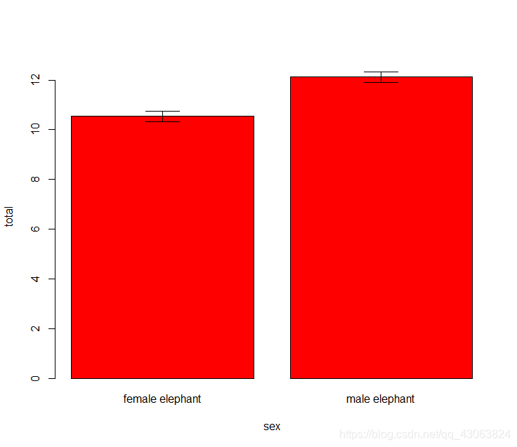
P-value is smaller than 0.05, accept the alternative hypothesis, the total tree-felling is different between sex.

Illustrate result of t-test

#Barplot of mean with error bars for standard error
mean.total = aggregate(list(total=elefell$total), by=list(sex=elefell$sex), mean, na.rm=TRUE)
SE = function(x) sd(x, na.rm=TRUE)/(sqrt(sum(!is.na(x))))
se.total = aggregate(list(SE=elefell$total), by=list(sex=elefell$sex), FUN=SE)
fell.dat = cbind(mean.total, SE=se.total$SE)
bp = barplot(total~sex, data=fell.dat, ylim = c(0, 13), col="red", names=c("female elephant", "male elephant"))
arrows(bp, fell.dat$total-fell.dat$SE, bp, fell.dat$total+fell.dat$SE, code=3, angle=90)

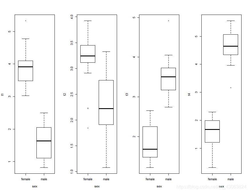
b) We can imagine that elephants might be more active at certain times of the day. Is there a difference in tree felling rates depending on time of day, and if so, is the relationship the same for both sexes? (5p)

According to the question, I use repeated measure here.

#Import data and check
elefell = read.csv('elefell.csv')
# plot data
par(mfrow=c(1,4))
boxplot(t1~sex, data = elefell)
boxplot(t2~sex, data = elefell)
boxplot(t3~sex, data = elefell)
boxplot(t4~sex, data = elefell)
par(mfrow=c(1,1))

#Construct Anova() model
fit = lm(cbind(t1,t2,t3,t4)~sex, data = elefell)
times = factor(c('t1','t2','t3','t4'))
fit.rep = Anova(fit, idata = data.frame(times), idesign=~times, type=3)

> #Check assumptions
> #Independent measurements
> dwtest(fit)

	Durbin-Watson test

data:  fit
DW = 2.2451, p-value = 0.7333
alternative hypothesis: true autocorrelation is greater than 0
# fullfiled

#Multivariate normality
> mvn(data = elefell[,2:5], mvnTest = 'mardia')
$multivariateNormality
             Test         Statistic           p value Result
1 Mardia Skewness  24.6357510253147 0.215723130397143    YES
2 Mardia Kurtosis 0.511592900269535 0.608935955379645    YES
3             MVN              <NA>              <NA>    YES

$univariateNormality
          Test  Variable Statistic   p value Normality
1 Shapiro-Wilk    t1        0.9341    0.0219    NO    
2 Shapiro-Wilk    t2        0.9502    0.0769    YES   
3 Shapiro-Wilk    t3        0.9375    0.0284    NO    
4 Shapiro-Wilk    t4        0.8806    0.0005    NO    

$Descriptives
    n     Mean   Std.Dev   Median       Min      Max     25th     75th        Skew   Kurtosis
t1 40 2.781751 1.3011629 2.761282 0.8136861 5.331051 1.651604 3.916465  0.04958455 -1.3456845
t2 40 2.742962 0.6978275 2.942996 1.0766608 3.924595 2.194925 3.264789 -0.39371416 -0.9033891
t3 40 2.668648 0.9611272 2.701272 1.2224455 4.917754 1.696224 3.487321  0.14425076 -1.1321676
t4 40 3.135586 1.6546084 2.732309 0.3083314 5.560109 1.687355 4.635793  0.01601791 -1.6852439

> mvn(data = elefell[,2:5], mvnTest = 'hz')
$multivariateNormality
           Test       HZ     p value MVN
1 Henze-Zirkler 1.099816 0.002596917  NO

$univariateNormality
          Test  Variable Statistic   p value Normality
1 Shapiro-Wilk    t1        0.9341    0.0219    NO    
2 Shapiro-Wilk    t2        0.9502    0.0769    YES   
3 Shapiro-Wilk    t3        0.9375    0.0284    NO    
4 Shapiro-Wilk    t4        0.8806    0.0005    NO    

$Descriptives
    n     Mean   Std.Dev   Median       Min      Max     25th     75th        Skew   Kurtosis
t1 40 2.781751 1.3011629 2.761282 0.8136861 5.331051 1.651604 3.916465  0.04958455 -1.3456845
t2 40 2.742962 0.6978275 2.942996 1.0766608 3.924595 2.194925 3.264789 -0.39371416 -0.9033891
t3 40 2.668648 0.9611272 2.701272 1.2224455 4.917754 1.696224 3.487321  0.14425076 -1.1321676
t4 40 3.135586 1.6546084 2.732309 0.3083314 5.560109 1.687355 4.635793  0.01601791 -1.6852439

> mvn(data = elefell[,2:5], mvnTest = 'royston')
$multivariateNormality
     Test        H     p value MVN
1 Royston 11.65649 0.002446813  NO

$univariateNormality
          Test  Variable Statistic   p value Normality
1 Shapiro-Wilk    t1        0.9341    0.0219    NO    
2 Shapiro-Wilk    t2        0.9502    0.0769    YES   
3 Shapiro-Wilk    t3        0.9375    0.0284    NO    
4 Shapiro-Wilk    t4        0.8806    0.0005    NO    

$Descriptives
    n     Mean   Std.Dev   Median       Min      Max     25th     75th        Skew   Kurtosis
t1 40 2.781751 1.3011629 2.761282 0.8136861 5.331051 1.651604 3.916465  0.04958455 -1.3456845
t2 40 2.742962 0.6978275 2.942996 1.0766608 3.924595 2.194925 3.264789 -0.39371416 -0.9033891
t3 40 2.668648 0.9611272 2.701272 1.2224455 4.917754 1.696224 3.487321  0.14425076 -1.1321676
t4 40 3.135586 1.6546084 2.732309 0.3083314 5.560109 1.687355 4.635793  0.01601791 -1.6852439

> mvn(data = elefell[,2:5], mvnTest = 'dh')
$multivariateNormality
            Test        E df   p value MVN
1 Doornik-Hansen 3.476949  8 0.9009713 YES

$univariateNormality
          Test  Variable Statistic   p value Normality
1 Shapiro-Wilk    t1        0.9341    0.0219    NO    
2 Shapiro-Wilk    t2        0.9502    0.0769    YES   
3 Shapiro-Wilk    t3        0.9375    0.0284    NO    
4 Shapiro-Wilk    t4        0.8806    0.0005    NO    

$Descriptives
    n     Mean   Std.Dev   Median       Min      Max     25th     75th        Skew   Kurtosis
t1 40 2.781751 1.3011629 2.761282 0.8136861 5.331051 1.651604 3.916465  0.04958455 -1.3456845
t2 40 2.742962 0.6978275 2.942996 1.0766608 3.924595 2.194925 3.264789 -0.39371416 -0.9033891
t3 40 2.668648 0.9611272 2.701272 1.2224455 4.917754 1.696224 3.487321  0.14425076 -1.1321676
t4 40 3.135586 1.6546084 2.732309 0.3083314 5.560109 1.687355 4.635793  0.01601791 -1.6852439

Pass ‘mardia’ and ‘dh’, the multivariate normality is fullfiled.

#Get results of repeated measures model using Anova()
> summary(fit.rep, multivariate=FALSE)

Univariate Type III Repeated-Measures ANOVA Assuming Sphericity

            Sum Sq num Df Error SS den Df  F value    Pr(>F)    
(Intercept) 555.00      1    8.796     38 2397.758 < 2.2e-16 ***
sex           6.29      1    8.796     38   27.188 6.787e-06 ***
times        74.35      3   34.862    114   81.041 < 2.2e-16 ***
sex:times   177.87      3   34.862    114  193.876 < 2.2e-16 ***
---
Signif. codes:  0 ‘***’ 0.001 ‘**’ 0.01 ‘*’ 0.05 ‘.’ 0.1 ‘ ’ 1


Mauchly Tests for Sphericity

          Test statistic p-value
times            0.86509 0.37805
sex:times        0.86509 0.37805


Greenhouse-Geisser and Huynh-Feldt Corrections
 for Departure from Sphericity

           GG eps Pr(>F[GG])    
times     0.92304  < 2.2e-16 ***
sex:times 0.92304  < 2.2e-16 ***
---
Signif. codes:  0 ‘***’ 0.001 ‘**’ 0.01 ‘*’ 0.05 ‘.’ 0.1 ‘ ’ 1

            HF eps   Pr(>F[HF])
times     1.002872 3.840346e-28
sex:times 1.002872 1.327803e-44

The Mauchly Tests for Sphericity is pass.

From the first table, time effect are significant which means there is a linear relationship between felling-rate and time. And significant interactions between the sex and time would indicate that the slope of the relationship between felling-rate and times different between sexes.

#Illustrate results
#Barplot of mean with error bars for standard error
mean.fell = aggregate(list(fell=elefell_new$fell), by=list(Time=elefell_new$Time,sex=elefell_new$sex), mean, na.rm=TRUE)
SE = function(x) sd(x, na.rm=TRUE)/(sqrt(sum(!is.na(x))))
se.fell = aggregate(list(SE=elefell_new$fell), by=list(Time=elefell_new$Time,sex=elefell_new$sex), FUN=SE)
fell.dat <-cbind(mean.fell, SE=se.fell$SE)
coefs = fit$coefficients
fell.mat = matrix(fell.dat$fell,4,2)
rownames(fell.mat) = c('early morning','late morning', 'early afternoon', 'late afternoon')
colnames(fell.mat) = c("Female", "Male")
bp <-barplot(fell.mat, beside = T, ylim=c(0, 6), col=c("red",'purple','green','orange'), names=c("Female elephant", "Male elephant"),legend=rownames(fell.mat))
arrows(c(bp[,1],bp[,2]), fell.dat$fell-fell.dat$SE, c(bp[,1],bp[,2]), fell.dat$fell+fell.dat$SE, code=3, angle=90)

c) What are the assumptions of the tests you carried out in parts a) and b)? (2p)

In part a), I used two-sample t-test, the assumptions are:

• felling data is independent
• the felling data for female and male elephant are both normally distributed.
• two groups data have similar variance.

In part b), I used Repeated measures, the assumptions are:

• Independent observations
• Multivariate normality
• Sphericity (multivariate homogeneity of variances)