ANN(MLP) 三种预测

目录

介绍： 

 一、Mlp for binary classification

数据： 

模型： 

预测：

二、Mlp for Multiclass Classification

数据：

模型：

预测：

三、MLP for Regression

数据：

模型： 

 预测：

介绍： 

多层感知器（Multilayer Perceptron，MLP）是一种基于人工神经网络的机器学习算法。它由多个神经元（也称为节点）组成，这些神经元排列在不同的层中，并且每个神经元都与上一层的神经元相连。

MLP的基本结构包括输入层、输出层和一个或多个隐藏层。输入层接收输入数据，输出层产生最终的输出结果。隐藏层在输入层和输出层之间，它们的作用是对输入数据进行抽象和特征提取。

每个神经元都有一个与之关联的权重，这些权重用于计算神经元的加权和。加权和经过激活函数的处理，最终产生神经元的输出。常见的激活函数包括Sigmoid函数、ReLU函数、Tanh函数等。激活函数的作用是引入非线性，以增加模型的表达能力。

MLP的训练过程主要涉及两个步骤：前向传播和反向传播。在前向传播中，输入数据通过网络，每个神经元计算加权和并通过激活函数传递给下一层。在反向传播中，根据网络输出和真实标签之间的误差，通过梯度下降法调整权重，以使预测结果尽可能接近真实值。

MLP可以用于分类和回归问题。在分类问题中，MLP可以通过输出层的激活函数（通常是Softmax函数）将输入数据映射到不同的类别。在回归问题中，MLP可以通过输出层的线性激活函数（通常是恒等函数）来预测连续值。

MLP具有一些优点，如能够学习复杂的非线性关系，适用于大量数据和特征的情况，并且能够处理缺失数据。但是，MLP也存在一些缺点，如对初始权重的依赖性，容易过拟合和计算复杂性较高。

总而言之，MLP是一种强大的机器学习算法，可以应用于各种任务，包括图像和语音识别、自然语言处理、推荐系统等。

 一、Mlp for binary classification

数据： 

# mlp for binary classification
from pandas import read_csv
from sklearn.model_selection import train_test_split
from sklearn.preprocessing import LabelEncoder
from tensorflow.keras import Sequential
from tensorflow.keras.layers import Dense
# load the dataset
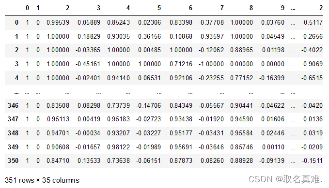
df = read_csv('ionosphere.csv', header=None)

 

模型： 

# split into input and output columns
X, y = df.values[:, :-1], df.values[:, -1]

# ensure all data are floating point values
X = X.astype('float32')

y = LabelEncoder().fit_transform(y)#改成0、1

# split into train and test datasets
X_train, X_test, y_train, y_test = train_test_split(X, y, test_size=0.33)
print(X_train.shape, X_test.shape, y_train.shape, y_test.shape)

# determine the number of input features
n_features = X_train.shape[1]

# define model
model = Sequential()#串型
model.add(Dense(10, activation='relu', kernel_initializer='he_normal', input_shape=(n_features,)))
model.add(Dense(8, activation='relu', kernel_initializer='he_normal'))
model.add(Dense(1, activation='sigmoid'))
# compile the model
model.compile(optimizer='adam', loss='binary_crossentropy', metrics=['accuracy'])

# fit the model
model.fit(X_train, y_train, epochs=150, batch_size=32, verbose=1)


# evaluate the model
loss, acc = model.evaluate(X_test, y_test, verbose=1)
print('Test Accuracy: %.3f' % acc)

预测：

# make a prediction
row = [1,0,0.99539,-0.05889,0.85243,0.02306,0.83398,-0.37708,1,0.03760,0.85243,-0.17755,0.59755,-0.44945,0.60536,-0.38223,0.84356,-0.38542,0.58212,-0.32192,0.56971,-0.29674,0.36946,-0.47357,0.56811,-0.51171,0.41078,-0.46168,0.21266,-0.34090,0.42267,-0.54487,0.18641,-0.45300]
yhat = model.predict([row])
print('Predicted: %.3f' % yhat)
if yhat >= 1/2: 
    yhat = 'G'
else:
    yhat = 'B'
print('Predicted: ', yhat)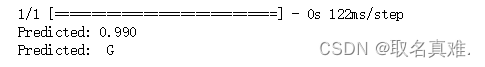

二、Mlp for Multiclass Classification

数据：

#ANN(MLP) for Multiclass Classification 预测蓝蝴蝶花品种 ('setosa', 'versicolor', 'virginica')
from numpy import argmax
import numpy as np
import matplotlib.pyplot as plt
import seaborn as sns; sns.set(style='white')
%matplotlib inline
from sklearn import decomposition
from sklearn import datasets

# Loading the dataset
iris = datasets.load_iris()
X = iris.data
y = iris.target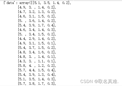

模型：

X_train, X_test, y_train, y_test = train_test_split(X, y, test_size=0.33)
print(X_train.shape, X_test.shape, y_train.shape, y_test.shape)
# determine the number of input features
n_features = X_train.shape[1]

# define model
model = Sequential()
model.add(Dense(10, activation='relu', kernel_initializer='he_normal', input_shape=(n_features,)))
model.add(Dense(8, activation='relu', kernel_initializer='he_normal'))
model.add(Dense(3, activation='softmax'))
# compile the model
model.compile(optimizer='adam', loss='sparse_categorical_crossentropy', metrics=['accuracy'])

# fit the model
model.fit(X_train, y_train, epochs=150, batch_size=32, verbose=1)

预测：

# evaluate the model
loss, acc = model.evaluate(X_test, y_test, verbose=0)
print('Test Accuracy: %.3f' % acc)
# make a prediction
row = [8.1,3.8,8.4,8.2]
#row = [2.1,3.5,3.4,2.2]
#row = [6.1,6.5,6.4,6.2]
yhat = model.predict([row])
print('Predicted: %s (class=%d)' % (yhat, argmax(yhat)))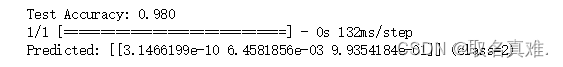

三、MLP for Regression

数据：

from numpy import sqrt
import pandas as pd
from sklearn.model_selection import train_test_split
from tensorflow.keras import Sequential
from tensorflow.keras.layers import Dense
# load the dataset
boston=pd.read_csv('boston.csv')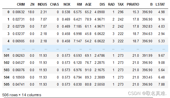

模型： 

y=boston["MEDV"]

X=boston.iloc[:,:-1]

# define model
model = Sequential()
model.add(Dense(10, activation='relu', kernel_initializer='he_normal', input_shape=(n_features,)))
model.add(Dense(8, activation='relu', kernel_initializer='he_normal'))
model.add(Dense(8, activation='relu', kernel_initializer='he_normal'))
model.add(Dense(1))
# compile the model
model.compile(optimizer='adam', loss='mse')
# fit the model
model.fit(X_train, y_train, epochs=150, batch_size=32, verbose=0)

#loss, acc = model.evaluate(X_test, y_test, verbose=0)
#print('Test Accuracy: %.3f' % acc)

# evaluate the model
error = model.evaluate(X_test, y_test, verbose=0)
print('MSE: %.3f, RMSE: %.3f' % (error, sqrt(error)))

 

 预测：

# make a prediction
row = [0.00632,18.00,2.310,0,0.5380,6.5750,65.20,4.0900,1,296.0,15.30,396.90,4.98]
yhat = model.predict([row])
print('Predicted: %.3f' % yhat)