Python学习--Machine-Learning 吴恩达机器学习编程作业 (第五周)

Machine-Learning 编程作业

Programming Exercise 5：Regularized Linear Regression and Bias v.s. Variance

正则化线性回归

1. 导入数据
2. 定义代价函数并将其正则化
3. 定义梯度函数并将其正则化
4. 利用高级函数进行优化，并画出拟合图

正则化线性回归

1. 导入数据，可视化

#!/usr/bin/env python
# -*- coding:utf-8 -*-
import numpy as np
import pandas as pd
import matplotlib.pyplot as plt
import seaborn as sns
import scipy.optimize as opt
from scipy.io import loadmat
import cv2 as cv

data = loadmat("ex5data1.mat")

#方法1取值：
X, y, Xval, yval, Xtest, ytest = map(np.ravel, [data['X'], data['y'], data['Xval'], data['yval'], data['Xtest'], data['ytest']])
#方法2取值：
# X = data['X']    #(12, 1)
# y = data['y']    #(12, 1)
# Xval = data['Xval']     #(21, 1)
# yval = data['yval']     #(21, 1)
# Xtest = data['Xtest']    #(21, 1)
# ytest = data['ytest']    #(21, 1)
print(X.shape, y.shape, Xval.shape, yval.shape, Xtest.shape, ytest.shape)

#方法1画图：
df = pd.DataFrame({ 'water_level':X , 'flow':y})
df.plot(x='water_level', y='flow', kind='scatter', figsize=(6,4))  #参见plot函数参数设置
plt.show()#画图
#方法2画图：
# sns.lmplot('water_level', 'flow', data=df, fit_reg=False, size=5)
# plt.show()

结果如下：

2. 定义代价函数并将其正则化
其代价函数根据练习文档中给出的定义，如下：

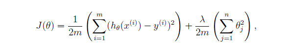
这里我们分成两部分，第一部分编写没有正则化项的代价函数，第二部分加上正则化项。

首先，初始化数据，给X，Xval， Xtest加上偏置项，并初始化theta。

#np.insert(arr,obj,values,axis) 插入的对象，位置，值，若axis=0则展平
X, Xval, Xtest = [np.insert(x.reshape(x.shape[0], 1), 0, np.ones(x.shape[0]), axis=1) for x in (X, Xval, Xtest)]
print(X)

#方法1的theta
theta = np.ones(X.shape[1])     #方法1的theta
#方法2：
# X = np.matrix(X)#将X的值转化为矩阵形式，方便计算
# y = np.matrix(y).T
# theta = np.matrix(np.ones(X.shape[1])).T

接下来是代价函数：

#定义代价函数
# 方法1：
def cost(theta, X, y):
    m = X.shape[0]
    inner = X @ theta - y  # R(m*1)
    square_sum = inner.T @ inner
    cost = square_sum / (2 * m)
    return cost
    
# 方法2：
# def cost(theta, X, y):
#     temp = np.power(((X * theta) - y), 2)
#     return np.sum(temp) / (2 * len(X))
# print(cost(theta, X, y))

#正则化代价函数
def r_cost(theta, X, y, l=1):
    r_term = (l / (2 * len(X))) * np.power(theta[1:], 2).sum()
    return cost(theta, X, y) + r_term
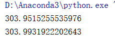
print(r_cost(theta, X, y))

结果如下，第一行是未经正则化的损失函数，第二行为正则化后的损失函数

3. 定义梯度函数并将其正则化
梯度函数公式：

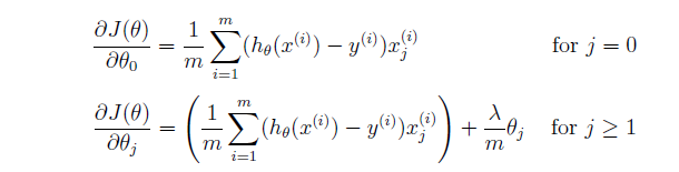
注意：偏置项没有进行正则化。
代码：

#定义梯度函数
# 方法1：
def gradient(theta, X, y):
    m = X.shape[0]
    inner = X.T @ (X @ theta - y)  # (m,n).T @ (m, 1) -> (n, 1)
    return inner / m
    
# #方法2：
# def gradient(theta, X, y):
#     print(theta.shape, X.shape, y.shape)
#     inner = X.T * ((X * theta) - y)
#     return inner / len(X)
#
print(gradient(theta, X, y))

#正则化梯度
def r_gradient(theta, X, y, l=1):
    r_term = theta.copy()  # same shape as theta
    r_term[0] = 0  # don't regularize intercept theta
    r_term = (l / len(X)) * r_term
    return gradient(theta, X, y) + r_term

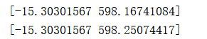
print(r_gradient(theta, X, y))

结果如下： 第一行未正则化，第二行经过正则化后

4. 利用高级函数进行优化，并画出拟合图

def linear_regression_np(X, y, l=1):
    theta = np.ones(X.shape[1])

    res = opt.minimize(fun=r_cost,
                       x0=theta,
                       args=(X, y, l),
                       method='TNC',
                       jac=r_gradient,
                       options={'disp': True})
    return res

theta = np.ones(X.shape[0])
final_theta = linear_regression_np(X, y, l=0).get('x')
print(final_theta)

#画图
b = final_theta[0] # intercept
m = final_theta[1] # slope
plt.scatter(X[:,1], y, label="Training data")
plt.plot(X[:, 1], X[:, 1]*m + b, label="Prediction")
plt.legend(loc=2)
plt.show()

结果如下：


第一部分到此结束。