Machine Learning-logistic regression

Machine Learning–logistic regression

我们拿到一大堆数据，然后根据这一大堆数据我们得到一个等式，来为我们做分类。

什么是 logistic regression

更适合用来做分类的sigmoid函数：

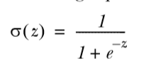
在 0 处值为 0.5， 增大趋近于 1， 减小趋近于 0

如果输入值 z 表示为w₀x₀+w₁x₁+ ······ w_nx_n （因为我们输入的 x 往往是一个 vector）需要考虑找到一个 w，也就是一个系数矩阵，并且应当是最佳的。

一些 optimization algorithms

gradient ascent 与 stochastic gradient ascent

梯度：

这时梯度上升就可以写成：

α 是步长， 后面乘的则是梯度方向，这样一来就总是得到函数的最大值

注意梯度算法的终止条件是：走特定的步数，或者到达特定的范围

def gradAscent(dataMatIn, classLabels):
    # dataMatrix 100 * 3, labelMat 1 * 100
    dataMatrix = mat(dataMatIn)
    # make labelMat to 100 * 1
    labelMat = mat(classLabels).transpose()
    m, n = shape(dataMatrix)
    alpha = 0.001
    # repeat times before stopping the calculation
    maxCycles = 500
    # start with all weights to 1, weights 3 * 1
    weights = ones((n, 1))
    for k in range(maxCycles):
        # calculate the gradient of the whole dataset, and h is a 100 * 1 matrix
        h = sigmoid(dataMatrix * weights)
        # calculate the error between predicted classes and actual classes
        error = (labelMat - h)
        # move in the direction of the error
        weights = weights + alpha * dataMatrix.transpose() * error
    return weights

最终返回一堆权重

前面的算法都是直接拿很多（一般是一定量）数据来做 traing，叫做 batch processing

stochastic gradient ascent 是一次一次计算 weights 来不断变化 weights， 它是 online learning algorithm

def stocGradAscent0(dataMatrix, classLabels):
    m, n = shape(dataMatrix)
    alpha = 0.01
    weights = ones((n))
    for i in range(m):
        h = sigmoid(sum(dataMatrix[i] * weights))
        error = classLabels[i] - h
        weights = weights + alpha * error * dataMatrix[i]
    return weights

不同之处在于这里全部用的是 array，没有 matrix， 这样操作就是基于 array 元素的了，是一个一个的了，不是一批一批的了

Action

gradient ascent:

stochastic gradient ascent:

看起来 stochastic gradient ascent 并没有什么优势，这是因为它只循环了一次。

def stocGradAscent1(dataMatrix, classLabels, numInter=150):
    m, n = shape(dataMatrix)
    weights = ones((n))
    for j in range(numInter):
        dataIndex = range(m)
        for i in range(m):
            alpha = 4 / (1.0 + j + i) + 0.01
            randIndex = int(random.uniform(0, len(dataIndex)))
            h = sigmoid(sum(dataMatrix[randIndex] * weights))
            error = classLabels[randIndex] - h
            weights = weights + alpha * error * dataMatrix[randIndex]
            del(dataIndex[randIndex])
    return weights

修改后的 stocGradAscent 加上了随机和循环次数

这是修改后的图形，已经要比之前的很好的了

# get the value of sigmoid and decide which this is a 1 or 0
def classifyVector(inX, weights):
    prob = sigmoid(sum(inX * weights))
    if prob > 0.5: return 1.0
    else: return 0.0

def colicTest():
    frTrain = open('horseColicTraining.txt')
    frTest = open('horseColicTest.txt')
    trainingSet = []
    trainingLabels = []
    for line in frTrain.readlines():
        # get each line

        currLine = line.strip().split('\t')
        lineArr = []
        for i in range(21):
            # get the list of lines

            lineArr.append(float(currLine[i]))
        trainingSet.append(lineArr)
        # get the labels of the data
        trainingLabels.append(float(currLine[21]))
    trainWeights = stocGradAscent1(array(trainingSet), trainingLabels, 1000)

    errorCount = 0;
    numTestVec = 0.0
    for line in frTest.readlines():
        numTestVec += 1.0
        currLine = line.strip().split('\t')
        lineArr = []
        for i in range(21):
            lineArr.append(float(currLine[i]))
        if int(classifyVector(array(lineArr), trainWeights)) != int(currLine[21]):
            errorCount += 1
    errorRate = (float(errorCount) / numTestVec)
    print("the error rate of this test is: %f" % errorRate)
    return errorRate

def multiTest():
    numTest = 10
    errorSum = 0.0
    for k in range(numTest):
        errorSum += colicTest()
    print("after %d iterations the average error rate is : %f"%(numTest, errorSum/float(numTest)))

最终计算出错误率。

那么 logistic regression 基本上到这儿为止，其基本原理是计算出预测值与标准值之间的偏差，然后修改权重，决定移动的方向