


学习NG的Machine Learning教程,先关推导及代码。由于在matleb或Octave中需要矩阵或向量,经常搞混淆,因此自己推导,并把向量的形式写出来了,主要包括cost function及gradient descent
见下图。
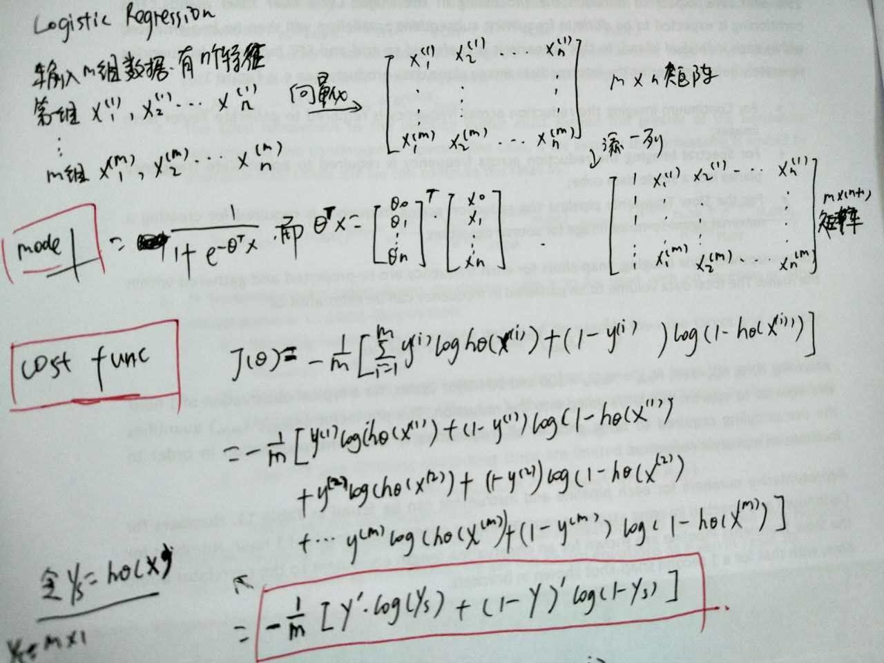
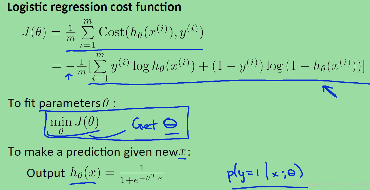
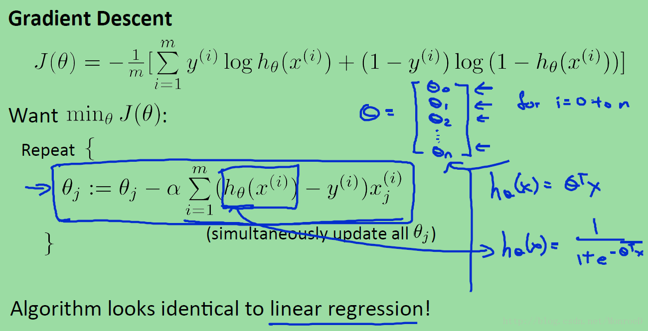
图中可见公式推导,及向量化表达形式的cost function(J)
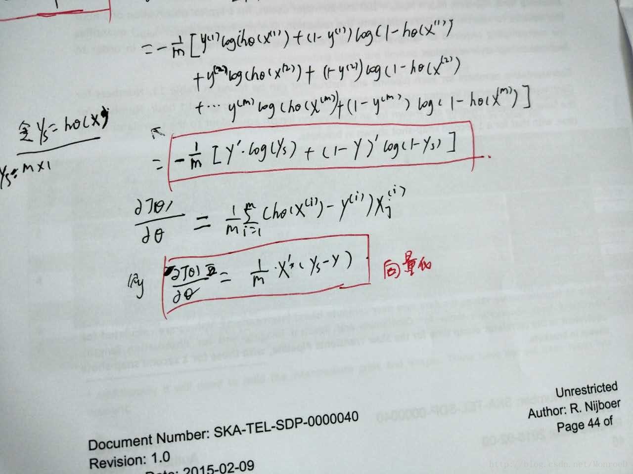
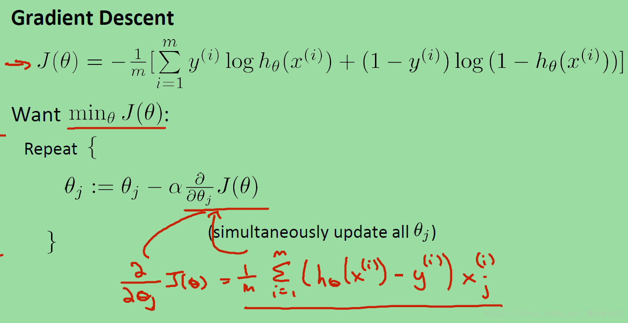
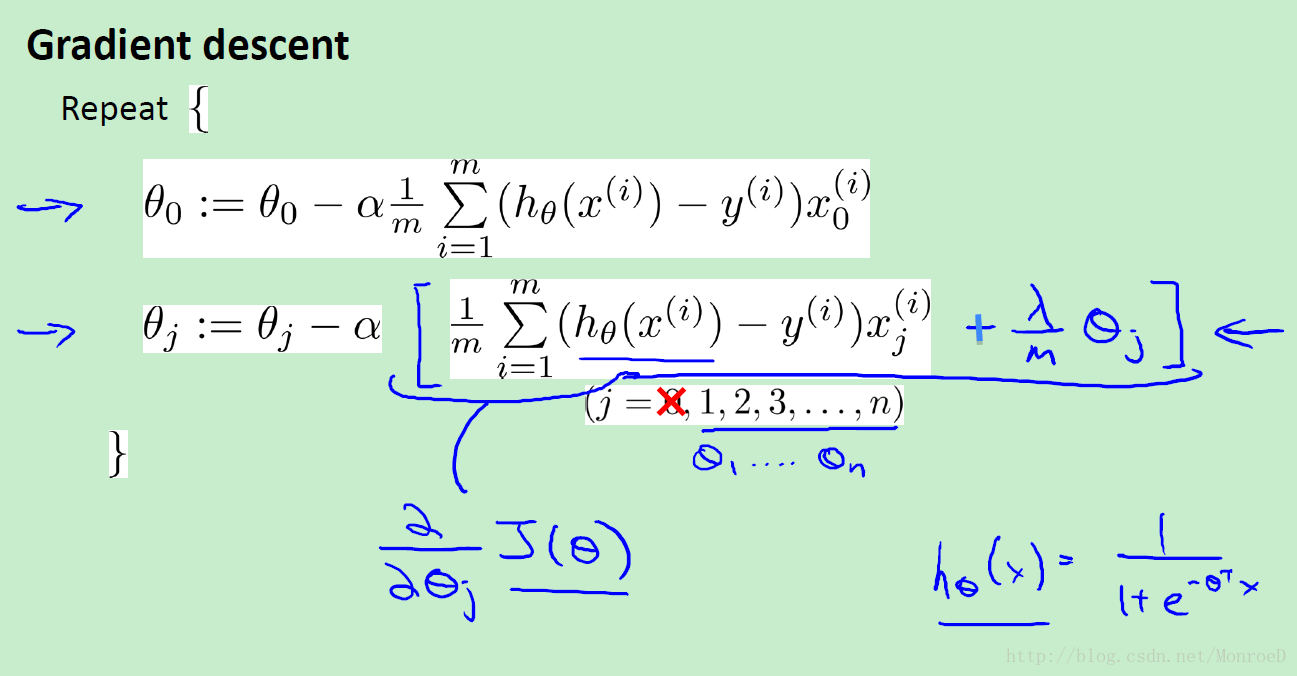
图中可见公式推导,及向量化表达形式的偏导数。
下面为Logistic regression的代码
data = load('ex2data1.txt');
X = data(:, [1, 2]); y = data(:, 3);

%% ==================== Part 1: Plotting ====================

fprintf(['Plotting data with + indicating (y = 1) examples and o ' ...
         'indicating (y = 0) examples.\n']);

plotData(X, y);

% Put some labels
hold on;
% Labels and Legend
xlabel('Exam 1 score')
ylabel('Exam 2 score')

% Specified in plot order
legend('Admitted', 'Not admitted')
hold off;

fprintf('\nProgram paused. Press enter to continue.\n');
pause;

%% ============ Part 2: Compute Cost and Gradient ============

%  Setup the data matrix appropriately, and add ones for the intercept term
[m, n] = size(X); % m:row n:col

% Add intercept term to x and X_test
X = [ones(m, 1) X];

% Initialize fitting parameters
initial_theta = zeros(n + 1, 1);

% Compute and display initial cost and gradient
[cost, grad] = costFunction(initial_theta, X, y);

pause;


%% ============= Part 3: Optimizing using fminunc  =============

%  Set options for fminunc
options = optimset('GradObj', 'on', 'MaxIter', 400);

%  Run fminunc to obtain the optimal theta
%  This function will return theta and the cost
[theta, cost] = ...
    fminunc(@(t)(costFunction(t, X, y)), initial_theta, options);

% Print theta to screen
fprintf('Cost at theta found by fminunc: %f\n', cost);
fprintf('theta: \n');
fprintf(' %f \n', theta);

% Plot Boundary
plotDecisionBoundary(theta, X, y);

% Put some labels
hold on;
% Labels and Legend
xlabel('Exam 1 score')
ylabel('Exam 2 score')

% Specified in plot order
legend('Admitted', 'Not admitted')
hold off;

fprintf('\nProgram paused. Press enter to continue.\n');
pause;

%% ============== Part 4: Predict and Accuracies ==============

prob = sigmoid([1 45 85] * theta);
fprintf(['For a student with scores 45 and 85, we predict an admission ' ...
         'probability of %f\n'], prob);

% Compute accuracy on our training set
p = predict(theta, X);

fprintf('Train Accuracy: %f\n', mean(double(p == y)) * 100);
fprintf('\n');
其中plotData的代码如下
function plotData(X, y)

% Create New Figure
figure; hold on;

pos = find(y==1); %
neg = find(y==0);

plot(X(pos,1), X(pos,2),'k+','LineWidth',2,'MarkerFaceColor','b');
plot(X(neg,1), X(neg,2),'yo','LineWidth',2,'MarkerFaceColor','y');

hold off;

end
其中costFunction的代码如下
function [J, grad] = costFunction(theta, X, y)

% Initialize some useful values
m = length(y); % number of training examples

J = 0;
grad = zeros(size(theta)); %(n+1)*1

ys = sigmoid(X*theta); % m*1
J = -1/m*(y'*log(ys) + (1-y)'*log(1-ys));
grad = 1/m*X'*(ys-y);

end
其中plotDecisionBoundary的代码如下
function plotDecisionBoundary(theta, X, y)
%PLOTDECISIONBOUNDARY Plots the data points X and y into a new figure with
%the decision boundary defined by theta
%   PLOTDECISIONBOUNDARY(theta, X,y) plots the data points with + for the
%   positive examples and o for the negative examples. X is assumed to be
%   a either
%   1) Mx3 matrix, where the first column is an all-ones column for the
%      intercept.
%   2) MxN, N>3 matrix, where the first column is all-ones

% Plot Data
plotData(X(:,2:3), y);
hold on

if size(X, 2) <= 3
    % Only need 2 points to define a line, so choose two endpoints
    plot_x = [min(X(:,2))-2,  max(X(:,2))+2];

    % Calculate the decision boundary line
    plot_y = (-1./theta(3)).*(theta(2).*plot_x + theta(1));

    % Plot, and adjust axes for better viewing
    plot(plot_x, plot_y)

    % Legend, specific for the exercise
    legend('Admitted', 'Not admitted', 'Decision Boundary')
    axis([30, 100, 30, 100])
else
    % Here is the grid range
    u = linspace(-1, 1.5, 50);
    v = linspace(-1, 1.5, 50);

    z = zeros(length(u), length(v));
    % Evaluate z = theta*x over the grid
    for i = 1:length(u)
        for j = 1:length(v)
            z(i,j) = mapFeature(u(i), v(j))*theta;
        end
    end
    z = z'; % important to transpose z before calling contour

    % Plot z = 0
    % Notice you need to specify the range [0, 0]
    contour(u, v, z, [0, 0], 'LineWidth', 2)
end
hold off

end
其中predit的代码如下
function p = predict(theta, X)

m = size(X, 1); % Number of training examples

p = zeros(m, 1);

p = X*theta;
for i = 1 : m
    if p(i) >= 0.5
        p(i) = 1;
    else
        p(i) = 0;
end

end
为方便查阅,将公式原图放下
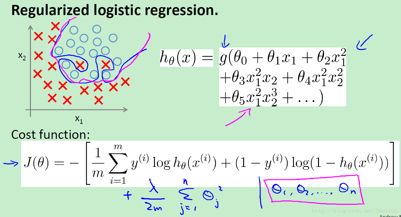
以下为regularization logistic regression


 221
221

 被折叠的 条评论
为什么被折叠?
被折叠的 条评论
为什么被折叠?
 到【灌水乐园】发言


