【图像处理】图像离散小波变换（Discrete Wavelet Transform）及python代码实现

Motivation

看到有论文用到了图像的Haar Discrete Wavelet Transform（HDWT），前面也听老师提到过用小波变换做去噪、超分的文章，于是借着这个机会好好学习一下。

直观理解

参考知乎上的这篇文章：https://zhuanlan.zhihu.com/p/22450818 关于傅立叶变换和小波变换的直观概念解释的非常清楚（需要对傅立叶变换有基本的理解）

二维图像离散小波变换（DWT）

先放一张图直观感受一下这个过程（图中是经过两次DWT的）
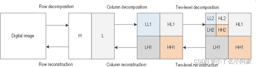
1. 首先明确什么是H和L。H和L其实表示的是高通滤波器（High pass filter）和低通滤波器（Low pass filter）。高通滤波器用于提取边缘特征，低通滤波器用于图像近似（approximation）.
2. 两次滤波得到输出结果。如下图所示，先通过低通和高通滤波器（纵向 vertical），再分别通过一次低通和高通滤波器（横向 horizontal）。最后得到LL, HL, LH, HH。分别表示近似图像（也可以理解为压缩了的图像，有损失）、纵向边缘特征（通过了纵向高通滤波器）、横向边缘特征（通过了横向高通滤波器）、对角特征（diagonal 横向纵向都通过高通滤波器）。

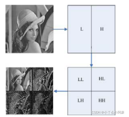
上图看不太清楚的话可以看下面这张图（看看后面的图就好了，中间的过程感觉表示的不太对）

来源：Wavelet based transition region extraction for image segmentation

关于横向和纵向的边缘特征，可以看下面这张有条纹噪声图片的HDWT(Haar Discrete Wavelet Transform)，比较明显。

来源： Wavelet Deep Neural Network for Stripe Noise Removal

python代码

import numpy as np
from matplotlib import pyplot as plt
import pywt
import PIL

img = PIL.Image.open("xxx.tif")
img = np.array(img)
LLY,(LHY,HLY,HHY) = pywt.dwt2(img, 'haar')
plt.subplot(2, 2, 1)
plt.imshow(LLY, cmap="Greys")
plt.subplot(2, 2, 2)
plt.imshow(LHY, cmap="Greys")
plt.subplot(2, 2, 3)
plt.imshow(HLY, cmap="Greys")
plt.subplot(2, 2, 4)
plt.imshow(HHY, cmap="Greys")
plt.show()

我的结果：

还是比较明显能看出水平和纵向特征的。

参考文章

1. https://medium.com/@koushikc2000/2d-discrete-wavelet-transformation-and-its-applications-in-digital-image-processing-using-matlab-1f5c68672de3
2. https://ataspinar.com/2018/12/21/a-guide-for-using-the-wavelet-transform-in-machine-learning/
3. https://medium.com/image-vision/2d-dwt-a-brief-intro-89e9ef1698e3

如果对您有帮助，请不要吝啬您的点赞，如需转载请评论告知！

在此谢过各位！