【机器学习】Nonlinear Independent Component Analysis - Aapo Hyvärinen

Linear independent component analysis (ICA)

$$x_i(k)=\sum _{j=1}^n{a}_{ij}{s}_j(k)\text{for all }i=1\dots n,k=1\dots K\text{\hspace{1em}()}$$

• $x_i(k)$ is the $i$-th observed signal in sample point $k$ (possibly time)
• $a_{ij}$ constant parameters describing “mixing”
• Assuming independent, non-Gaussian latent “sources” $s_j$
• ICA is identifiable, i.e. well-defined. Observing only $x_i$ we can recover both $a_{ij}$ and $s_j$ .

Fundamental difference between ICA and PCA

• PCA doesn’t find the original coordinates, ICA does.

• PCA, Gaussian factor analysis are not identifiable:
  • Any orthogonal rotation is equivalent: $s^{\prime }=Us$ has same distribution.

Nonlinear ICA is an unsolved problem

• Extend ICA to nonlinear case to get general disentanglement?

• Unfortunately, “basic” nonlinear ICA is not identifiable:

• If we define nonlinear ICA model for random variables ( x_i ) as

  $$x_i=f_i(s_1,\dots ,s_n),i=1\dots n$$

  we cannot recover original sources (Darmois, 1952; Hyvärinen & Pajunen, 1999)

Darmois construction

• Darmois (1952) showed the impossibility of nonlinear ICA:

• For any $x_1,x_2$, can always construct $y=g(x_1,x_2)$ independent of $x_1$ as

  $$g({\xi }_1,{\xi }_2)=P(x_2<{\xi }_2|x_1={\xi }_1)$$

• Independence alone too weak for identifiability:

  • We could take $x_1$ as an independent component which is absurd

• Looking at non-Gaussianity equally absurd:

  • Scalar transform $h(x_1)$ can give any distribution

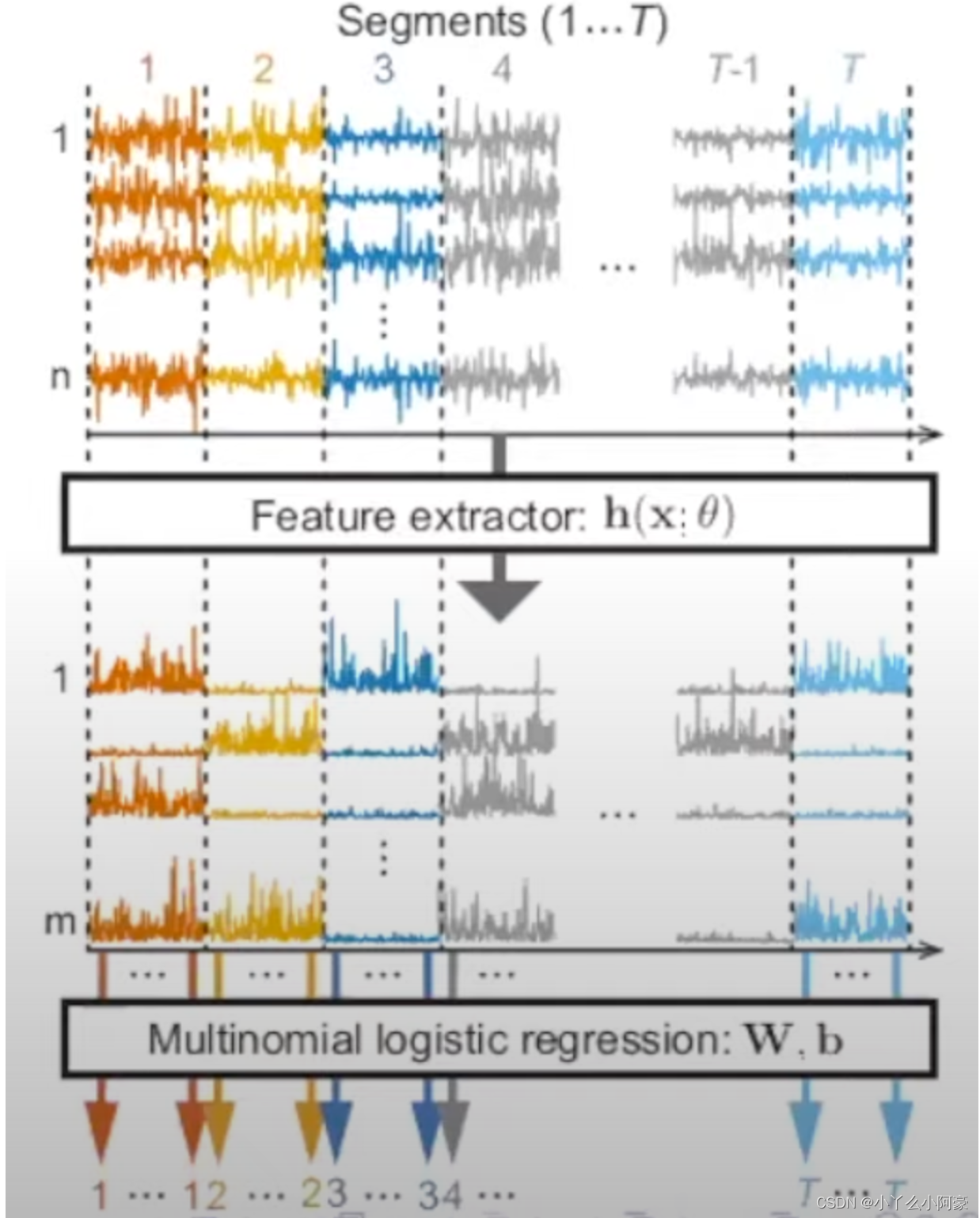
Time-contrastive learning

• Observe $n$-dim time series $x(t)$
• Divide $x(t)$ into $T$ segments (e.g., bins with equal sizes)
• Train MLP to tell which segment a single data point comes from
  • Number of classes is $T$
  • Labels given by index of segment
  • Multinomial logistic regression
• In hidden layer $h$, NN should learn to represent nonstationarity 非平稳性 (= differences between segments)
• Could this really do Nonlinear ICA?

• Assume data follows nonlinear ICA model $x(t)=f(s(t))$ with
  • smooth, invertible nonlinear mixing $f:{\mathbb{R}}^n\to {\mathbb{R}}^n$
  • components $s_i(t)$ are nonstationary, e.g., in variances
• Assume we apply time-contrastive learning on $x(t)$
  • using MLP with hidden layer in $h(x(t))$ with $\text{dim}(h)=\text{dim}(x)$
• Then, TCL will find $s(t{)}^2=Ah(x(t))$ for some linear mixing matrix $A$. (Squaring is element-wise)
• I.e.: TCL demixes nonlinear ICA model up to linear mixing (which can be estimated by linear ICA) and up to squaring.
• This is a constructive proof of identifiability
• Imposing independence at every segment -> more constraints -> unique solution. 增加了限制保证了indentifiability

用MLP，通过自监督分类（某一个信号来自于哪个时间段）来训练网络。这样MLP可以表示不同时间段内的信号差。而后原始信号 $s^2$ 可以表示为观测值(x)经MLP隐藏层分离结果的线性组合。

Deep Latent Variable Models

• General framework with observed data vector $x$ and latent $s$:
  $$p(x,s)=p(x|s)p(s),p(x)=\int p(x,s)ds$$
  where $\theta$ is a vector of parameters, e.g., in a neural network

• In variational autoencoders (VAE):

  • Define prior so that $s$ white Gaussian (thus $s_i$; all independent)
  • Define posterior so that $x=f(s)+n$

• Looks like Nonlinear ICA, but not identifiable

  • By Gaussianity, any orthogonal rotation is equivalent:
    $$s^{\prime }=Ms\text{ has exactly the same distribution if }{M}^{T}M=I$$

Conditioning DLVM’s by another variable

通过引入一个新的变量u来解，比如找视频和音频的关系，时间t就可以作为辅助变量（auxiliary varibale）。通过条件独立（conditional independent）来解。

Conclusion

• Typical deep learning needs class labels, or some targets

• If no class labels: unsupervised learning

• Independent component analysis is a principled approach

  • can be made nonlinear

• Identifiable: Can recover components that actually created the data (unlike PCA, VAE etc)

• Special assumptions needed for identifiability, one of:

  • Nonstationarity (“time-contrastive learning”)
  • Temporal dependencies (“permutation-contrastive learning”)
  • Existence of auxiliary (conditioning) variable (e.g., “iVAE”)

• Self-supervised methods are easy to implement

• Connection to DLVM’s can be made → iVAE

• Principled framework for “disentanglement”

总结来说Linear ICA是可解的，对于Nonlinear ICA则需要增加额外的假设才能可解（原始信号可分离）。Nonlinear ICA的思想可以用在深度学习的其他模型上。

Reference

1. https://www.youtube.com/watch?v=_cBLSNRWt8c