


ViT:AN IMAGE IS WORTH 16X16 WORDS: TRANSFORMERS FOR IMAGE RECOGNITION AT SCALE——ICLR,2021
Pytroch代码来源:https://github.com/lucidrains/vit-pytorch
一、背景介绍
目前在NLP领域,transformer已经占据主导地位。不少学者尝试将attention和CNN相结合,这些方法往往依赖于CNN,其性能相较于常见的卷积网络如ResNet等还是有差别。但是使用VIT能够解决许多CNN不能解决的问题。
在NLP领域,使用transformer时,当不断增加模型大小和数据集数量,模型性能没有出现饱和趋势。同样的在CV领域,当数据量较小时,使用transformer有时并不比常见卷积性能好。但当数据集数量不断变大,transformer性能不断提高,甚至超过常见卷积模型。
二、方法介绍
本片论文介绍的方法主要是用来进行分类的。输入一张图片,输出特征。作者在结论中也说到,本文方法的一个挑战是如何把ViT应用到检测和分割等视觉任务上。作者的动机是尽可能减少Transformer原始结构的改变。ViT的输入是将图像块通过线性映射从2d图像块变成1d序列。作者在介绍中说到,ViT在中小规模数据集上的表现性能有时还不如卷积网络,但当使用大规模数据集时,性能就会超过卷积网络。
因为论文内容写的比较简单,而本篇博客主要是为了熟悉并学习如何使用ViT,故需要结合相关代码(代码为网上找的Pytroch版本,不是作者提供的源码,仅供参考)。
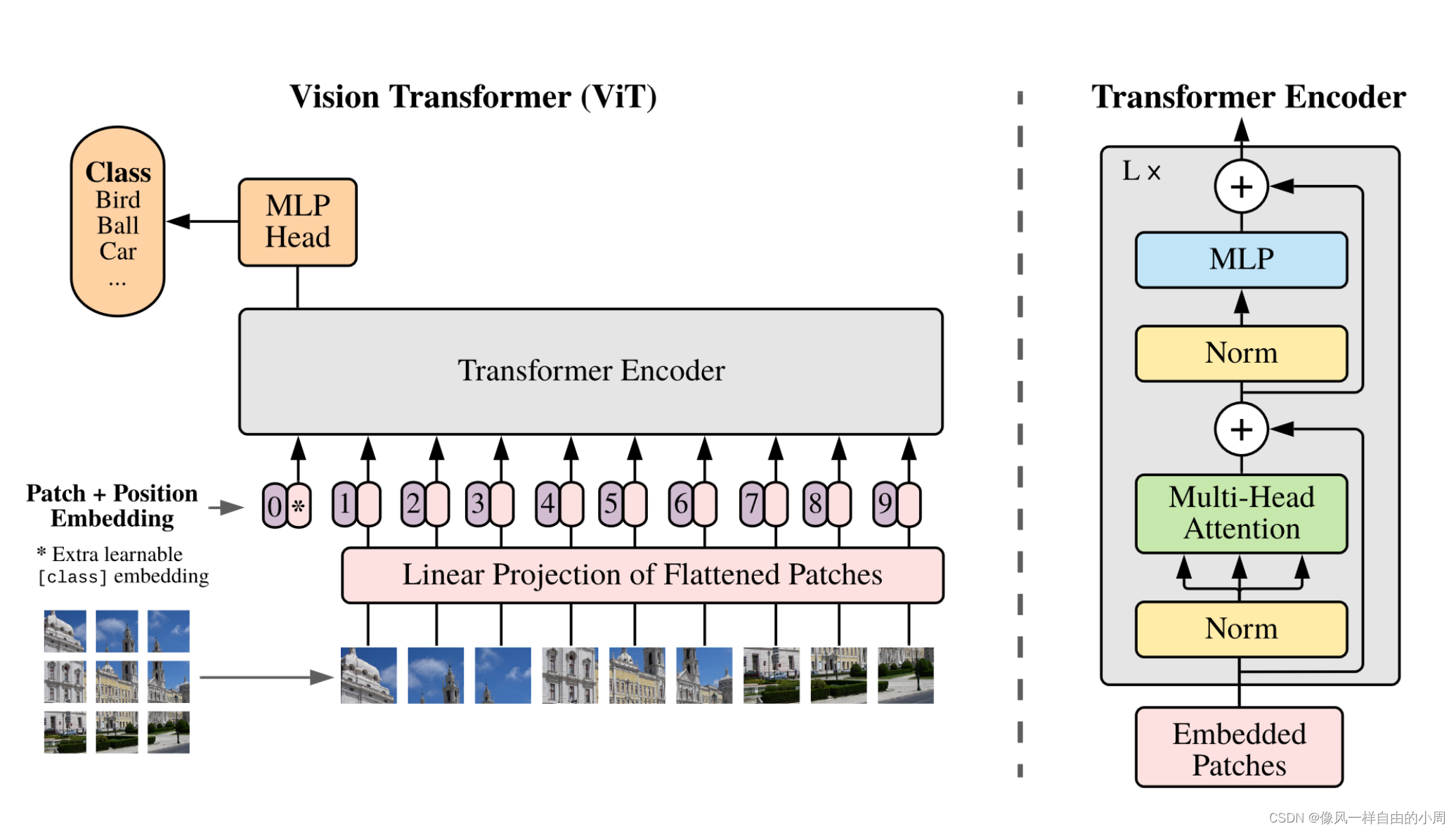
首先,本文结构如果熟悉Transformer的话是比较容易理解的。基本流程为先将图像大小为 x ∈ R H × W × C x\in R^{H\times W \times C} x∈RH×W×C裁剪成相同大小没有重叠部分的patch块, x p ∈ R ( N × ( P 2 ⋅ C ) ) x_p\in R^{(N \times (P^2 \cdot C))} xp∈R(N×(P2⋅C)),其中 H W = N P 2 HW=NP^2 HW=NP2, ( P , P ) (P,P) (P,P)为裁剪出的patch大小。然后将patch块通过线性映射变成 x p a t c h ∈ R D x_{patch}\in R^D xpatch∈RD。
这里的线性映射的代码如下,其中关于einops库中的rearrange相关介绍可以参考einops.rearrange:
from einops.layers.torch import Rearrange

self.to_patch_embedding = nn.Sequential(
            Rearrange('b c (h p1) (w p2) -> b (h w) (p1 p2 c)', p1 = patch_height, p2 = patch_width),
            nn.LayerNorm(patch_dim),
            nn.Linear(patch_dim, dim),
            nn.LayerNorm(dim), # dim=D
        )
接着和BERT做法一样添加[class] token
x
c
l
a
s
s
x_{class}
xclass,
x
c
l
a
s
s
x_{class}
xclass就不需要通过线性映射层了,这是一个可学习参数,Pytroch中直接令self.cls_token = nn.Parameter(torch.randn(1, 1, dim)),其中
d
i
m
=
D
dim=D
dim=D。
这里的 x c l a s s x_{class} xclass通过Transformer encoder之后得到 y y y就是最终的输出结果。
Transformer中用到了位置编码,这里作者使用了1D位置编码,因为作者通过实验发现使用2D位置编码,效果并未得到较大的提升。这里就比较有意思了,论文中作者说这个位置信息是学出来的,而不是一开始就给定的(像1,2,3,。。。这样的位置编码)。为啥要加位置编码呢?李沐在B站上这样解释:因为图片是有位置信息的,如果Patch块位置互换就不是原来的图片了,这都不是原来图片了,训练还有啥意思。
self.pos_embedding = nn.Parameter(torch.randn(1, num_patches + 1, dim)) # 这里的位置编码采用的是可学习编码
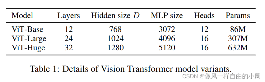
接下来便是Transformer Encoder的结构,包含multiheaded self-attention(MSA)和MLP blocks。每一层中都添加了Layernorm(LN)层,并采用了residual connection。Transformer Encoder中的每一个block输入序列为197x768,输出还是197x768,就是输入输出维度一样(假设输入图片大小为224x224,patch大小为16x16,则有14x14=196个patch,通过线性映射得到196个序列长度,加上class token和位置编码便变成了197个序列长度,dim=D=768=16x16x3,这里的3是通道数)。代码如下:
import torch
from torch import nn

from einops import rearrange, repeat
from einops.layers.torch import Rearrange

# helpers

def pair(t):
    return t if isinstance(t, tuple) else (t, t)

# classes

class PreNorm(nn.Module):
    def __init__(self, dim, fn):
        super().__init__()
        self.norm = nn.LayerNorm(dim)
        self.fn = fn
    def forward(self, x, **kwargs):
        return self.fn(self.norm(x), **kwargs)

class FeedForward(nn.Module):
    def __init__(self, dim, hidden_dim, dropout = 0.):
        super().__init__()
        self.net = nn.Sequential(
            nn.Linear(dim, hidden_dim),
            nn.GELU(),
            nn.Dropout(dropout),
            nn.Linear(hidden_dim, dim),
            nn.Dropout(dropout)
        )
    def forward(self, x):
        return self.net(x)

class Attention(nn.Module):
    def __init__(self, dim, heads = 8, dim_head = 64, dropout = 0.):
        super().__init__()
        inner_dim = dim_head *  heads
        project_out = not (heads == 1 and dim_head == dim)

        self.heads = heads
        self.scale = dim_head ** -0.5

        self.attend = nn.Softmax(dim = -1)
        self.dropout = nn.Dropout(dropout)

        self.to_qkv = nn.Linear(dim, inner_dim * 3, bias = False)

        self.to_out = nn.Sequential(
            nn.Linear(inner_dim, dim),
            nn.Dropout(dropout)
        ) if project_out else nn.Identity()

    def forward(self, x):
        qkv = self.to_qkv(x).chunk(3, dim = -1)
        q, k, v = map(lambda t: rearrange(t, 'b n (h d) -> b h n d', h = self.heads), qkv)

        dots = torch.matmul(q, k.transpose(-1, -2)) * self.scale

        attn = self.attend(dots)
        attn = self.dropout(attn)

        out = torch.matmul(attn, v)
        out = rearrange(out, 'b h n d -> b n (h d)')
        return self.to_out(out)

class Transformer(nn.Module):
    def __init__(self, dim, depth, heads, dim_head, mlp_dim, dropout = 0.):
        super().__init__()
        self.layers = nn.ModuleList([])
        for _ in range(depth):
            self.layers.append(nn.ModuleList([
                PreNorm(dim, Attention(dim, heads = heads, dim_head = dim_head, dropout = dropout)),
                PreNorm(dim, FeedForward(dim, mlp_dim, dropout = dropout))
            ]))
    def forward(self, x):
        for attn, ff in self.layers:
            x = attn(x) + x
            x = ff(x) + x
        return x
接下来便是ViT的整体实现了。可以看到,这个类的输入的batch里面均为整张图片。因为做的是分类任务,不能直接把Transformer block的输出作为最终结果,需要添加一个线性分类头。而Transformer block输出的序列个数是很多的,作者这里借鉴了NLP领域的做法,直接使用class token的输出作为预测结果(代码中还有另一种做法就是使用均值)。为啥能够这样做呢?是因为通过Attention,各个特征之间能够较好的交互。
class ViT(nn.Module):
    def __init__(self, *, image_size, patch_size, num_classes, dim, depth, heads, mlp_dim, pool = 'cls', channels = 3, dim_head = 64, dropout = 0., emb_dropout = 0.):
        super().__init__()
        image_height, image_width = pair(image_size)
        patch_height, patch_width = pair(patch_size)

        assert image_height % patch_height == 0 and image_width % patch_width == 0, 'Image dimensions must be divisible by the patch size.'

        num_patches = (image_height // patch_height) * (image_width // patch_width)
        patch_dim = channels * patch_height * patch_width
        assert pool in {'cls', 'mean'}, 'pool type must be either cls (cls token) or mean (mean pooling)'

        self.to_patch_embedding = nn.Sequential(
            Rearrange('b c (h p1) (w p2) -> b (h w) (p1 p2 c)', p1 = patch_height, p2 = patch_width),
            nn.LayerNorm(patch_dim),
            nn.Linear(patch_dim, dim),
            nn.LayerNorm(dim),
        )

        self.pos_embedding = nn.Parameter(torch.randn(1, num_patches + 1, dim))
        self.cls_token = nn.Parameter(torch.randn(1, 1, dim))
        self.dropout = nn.Dropout(emb_dropout)

        self.transformer = Transformer(dim, depth, heads, dim_head, mlp_dim, dropout)

        self.pool = pool
        self.to_latent = nn.Identity()

        self.mlp_head = nn.Sequential(
            nn.LayerNorm(dim),
            nn.Linear(dim, num_classes)
        )

    def forward(self, img):
        x = self.to_patch_embedding(img)
        b, n, _ = x.shape

        cls_tokens = repeat(self.cls_token, '1 1 d -> b 1 d', b = b)
        x = torch.cat((cls_tokens, x), dim=1)
        x += self.pos_embedding[:, :(n + 1)]
        x = self.dropout(x)

        x = self.transformer(x)

        x = x.mean(dim = 1) if self.pool == 'mean' else x[:, 0] # 这里代码实现又两个选择,一个是取所有patch块提取特征的均值,另一个是和论文中的一样取[class] token

        x = self.to_latent(x)
        return self.mlp_head(x)
论文中给出的计算公式如下,其中 z L 0 z_L^0 zL0:表示的是 x c l a s s x_{class} xclass通过多层Transformer输出的特征。

作者在这里还提出了一种混合框架(Hybrid Architecture),即输入的不是图像而是通过CNN提取的图像特征。
如果想要使用ViT作为特征提取器,可以把最后一层的mlp_head去掉,添加下游任务的头。通过预训练等方式进行微调即可。
微调: 不同尺寸图片进行微调的话,因为位置编码是提前预训练好的,尺寸固定住了,作者的一个解决方式是使用插值。
三、实验结果
1.使用class token做分类和GAP之间的区别
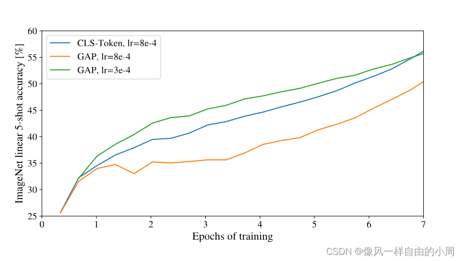
通过实验作者发现,都可以。这图泪目了,调参很重要。
2.不同的位置编码

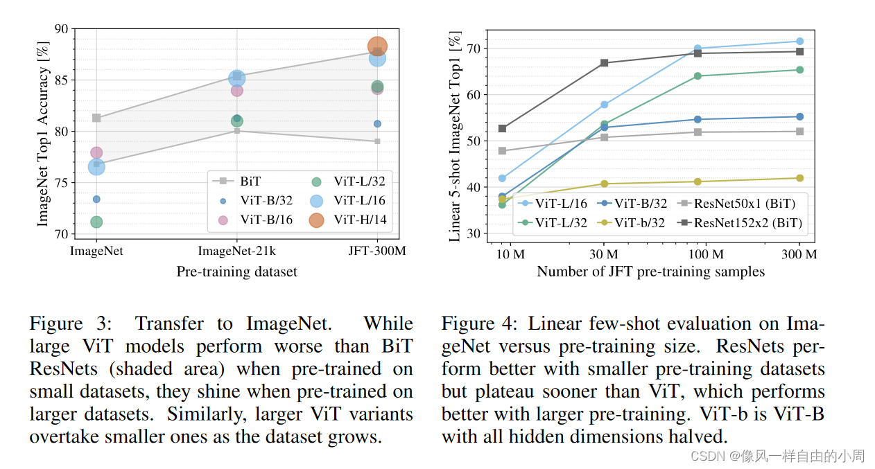
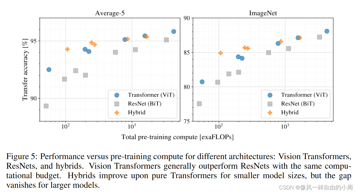
3.对比实验

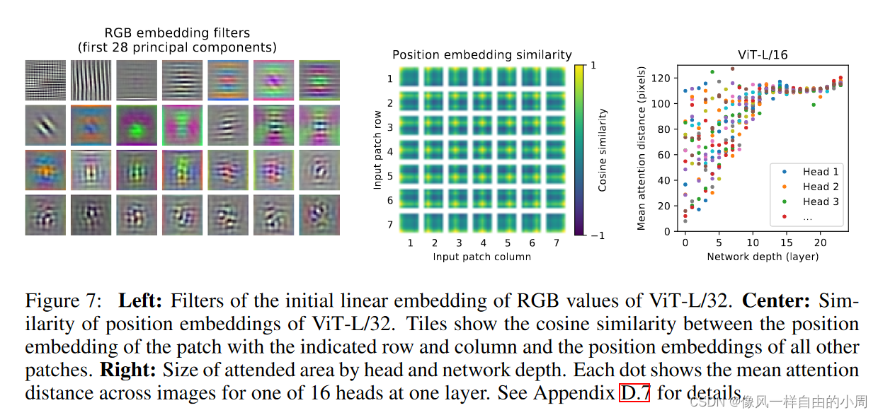
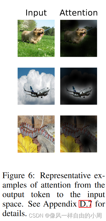
4.特征可视化


 339
339


 被折叠的 条评论
为什么被折叠?
被折叠的 条评论
为什么被折叠?
 到【灌水乐园】发言


