Improving Deep Neural Networks —— 第二周笔记

1. batch vs. mini-batch
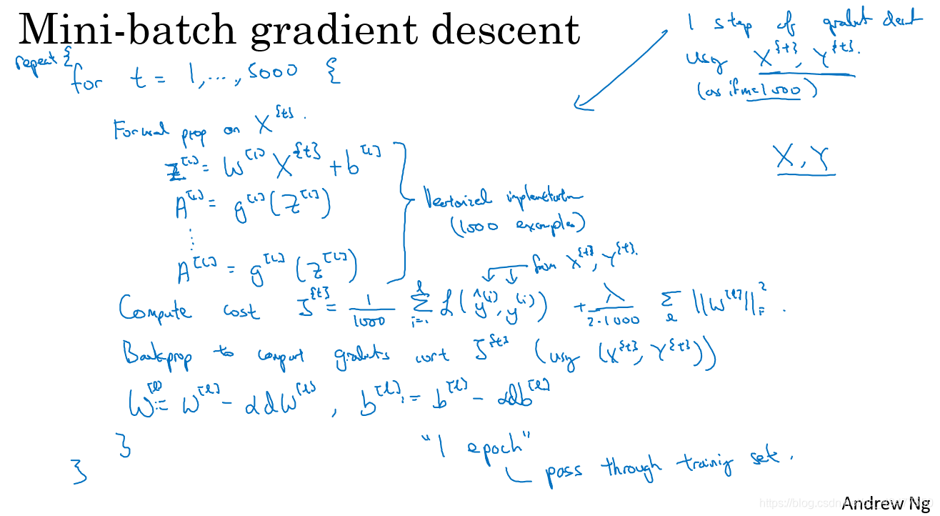
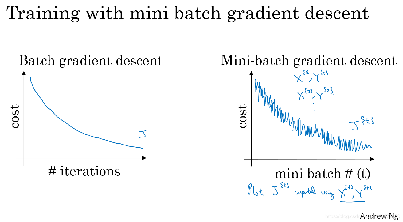
   batch指遍历完全部的数据集之后再进行梯度下降的方法，mini-batch是将数据集分成若干小的子集，分别进行梯度下降，这样可以提升速度。
   
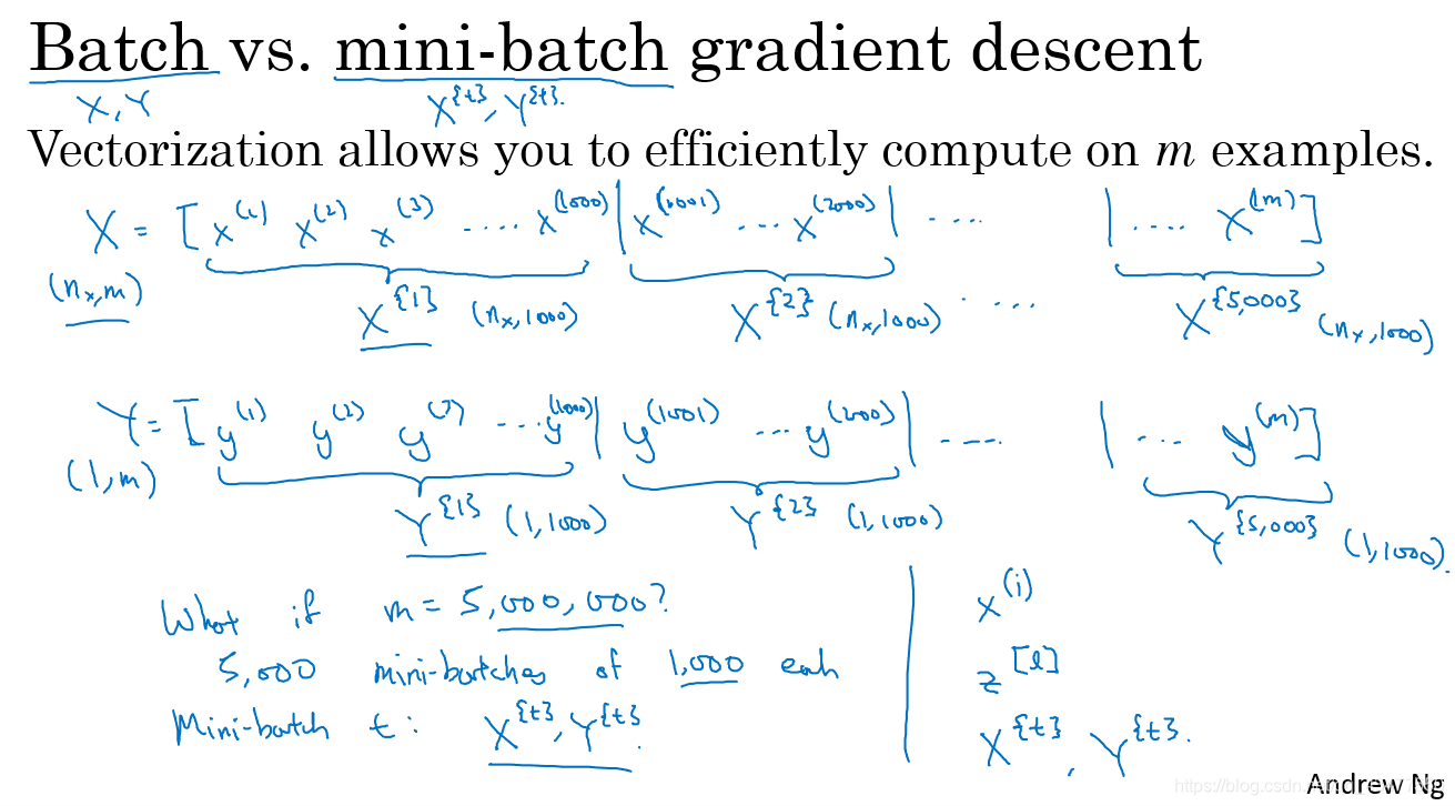
   epoch表示遍历完一整个训练集，当使用batch梯度下降时，1个epoch只进行了1次梯度下降，当使用mini-batch时，1个epoch可以进行t次梯度下降。
   
2. mini-batch size 的选择
   
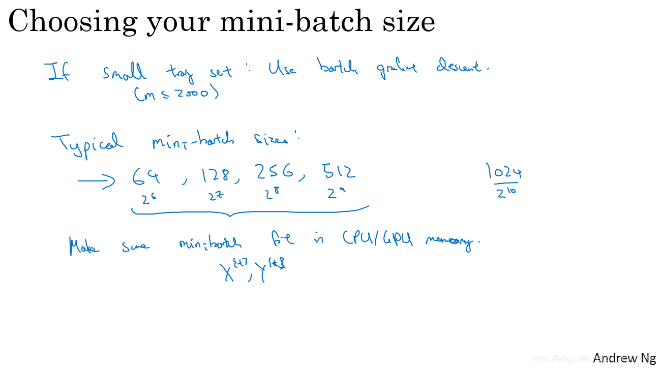
   mini-batch size = m时，为batch gradient descent 缺点：耗时长
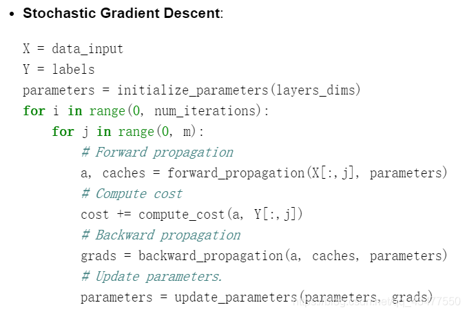
   mini-batch size = 1时，为stochastic gradient descent （随机梯度下降）缺点：丢失了向量化带来的加速。并且永远不会收敛，只会在最小值附近徘徊。
   所以先择中间值比较好。
   
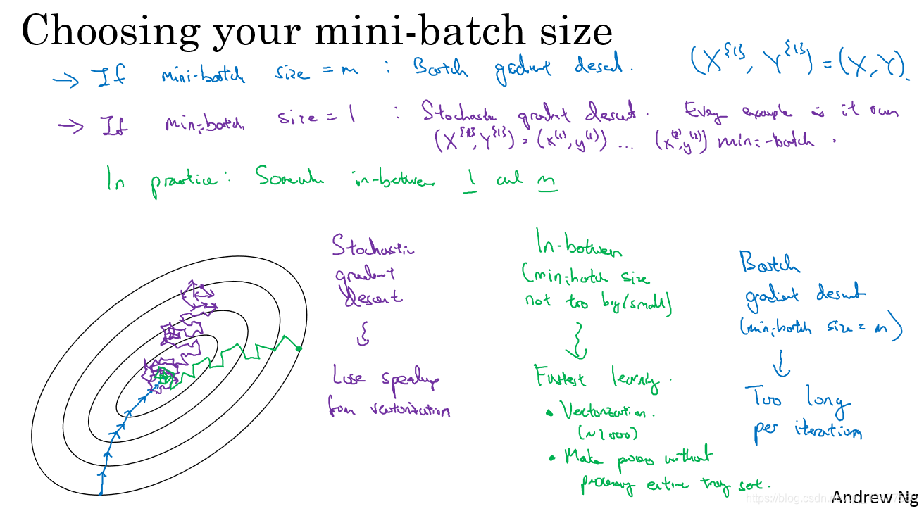
   当m<2000时，选择batch gradient descent
   当m>2000时，使用mini——batch gradient descent，大小一般为2的倍数，64，256，512等。
   需要注意的是，size的大小要和cpu/gpu的内存相匹配。
   
   
   mini-batch要经过两步
   （1）shuffle

permutation = list(np.random.permutation(m))
shuffled_X = X[:, permutation]
shuffled_Y = Y[:, permutation].reshape((1,m))

（2）Partition

num_complete_minibatches = math.floor(m/mini_batch_size) # number of mini batches of size mini_batch_size in your partitionning
for k in range(0, num_complete_minibatches):
    ### START CODE HERE ### (approx. 2 lines)
    mini_batch_X = shuffled_X[:,k*mini_batch_size:(k+1)*mini_batch_size]
    mini_batch_Y = shuffled_Y[:,k*mini_batch_size:(k+1)*mini_batch_size].reshape((1,-1))
    ### END CODE HERE ###
    mini_batch = (mini_batch_X, mini_batch_Y)
    mini_batches.append(mini_batch)

# Handling the end case (last mini-batch < mini_batch_size)
if m % mini_batch_size != 0:
    ### START CODE HERE ### (approx. 2 lines)
    mini_batch_X = shuffled_X[:,num_complete_minibatches*mini_batch_size:m]
    mini_batch_Y = shuffled_Y[:,num_complete_minibatches*mini_batch_size:m].reshape((1,-1))
    ### END CODE HERE ###
    mini_batch = (mini_batch_X, mini_batch_Y)
    mini_batches.append(mini_batch)

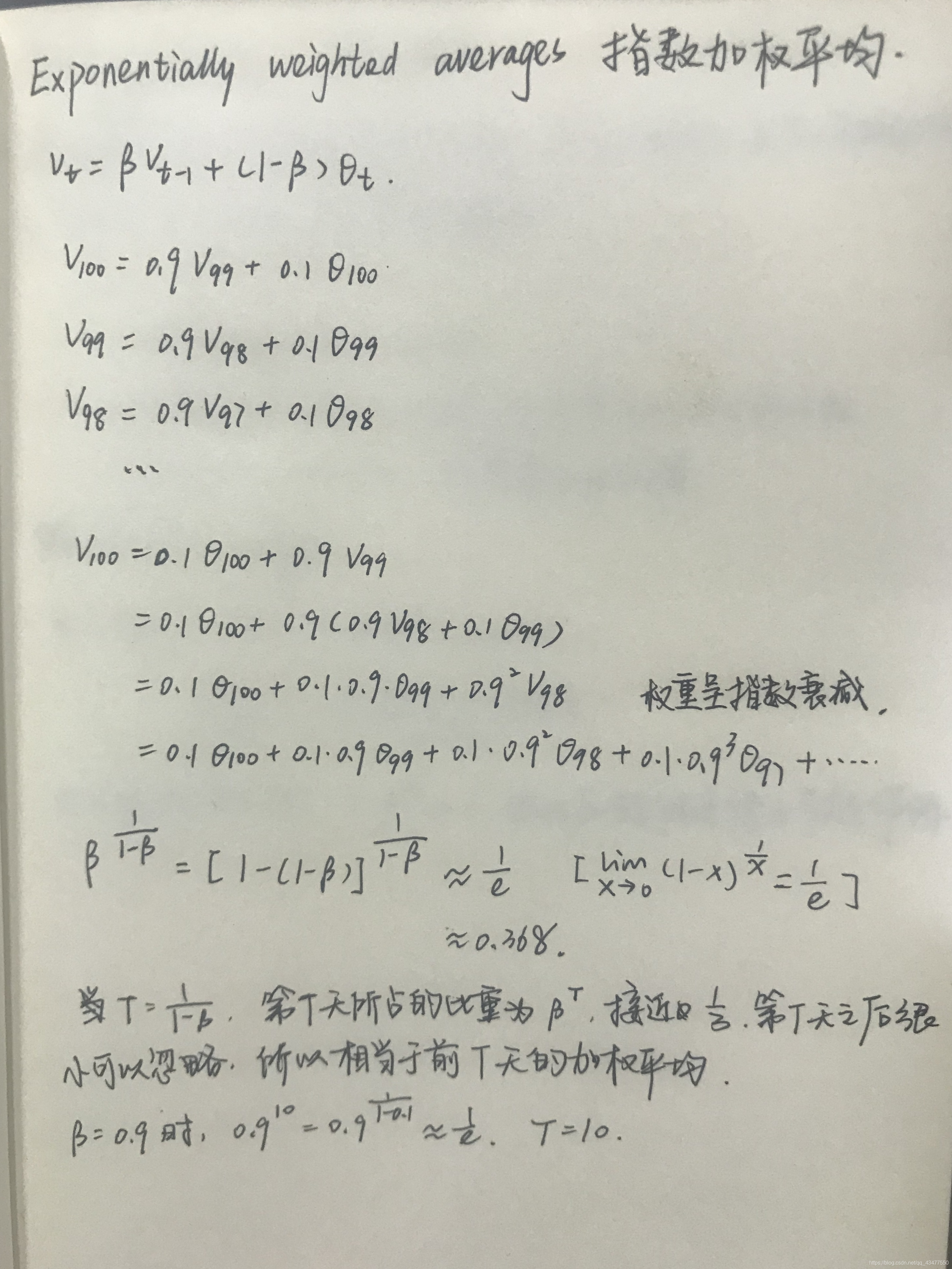
3. 指数加权移动平均 Exponentially Weighted Moving Averages
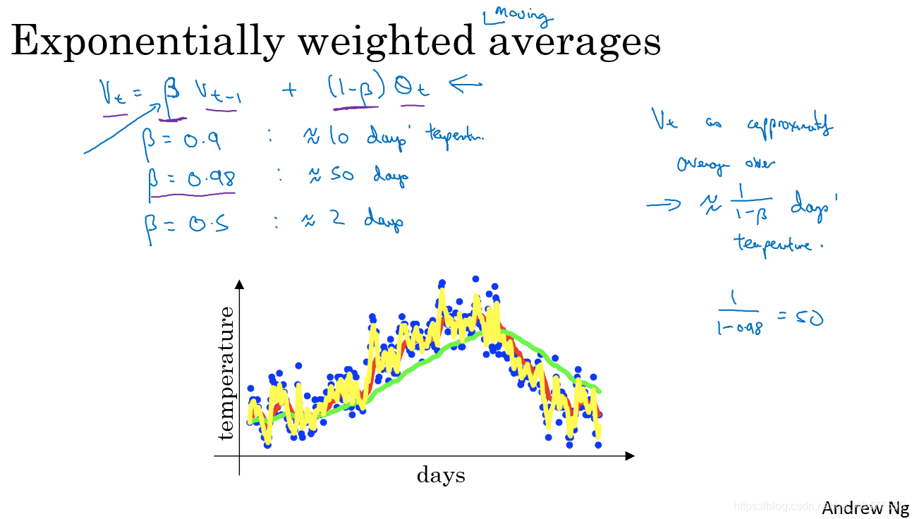   vt表示当天的温度平均值约等于前T天温度数据加权平均，T≈1/(1-β).

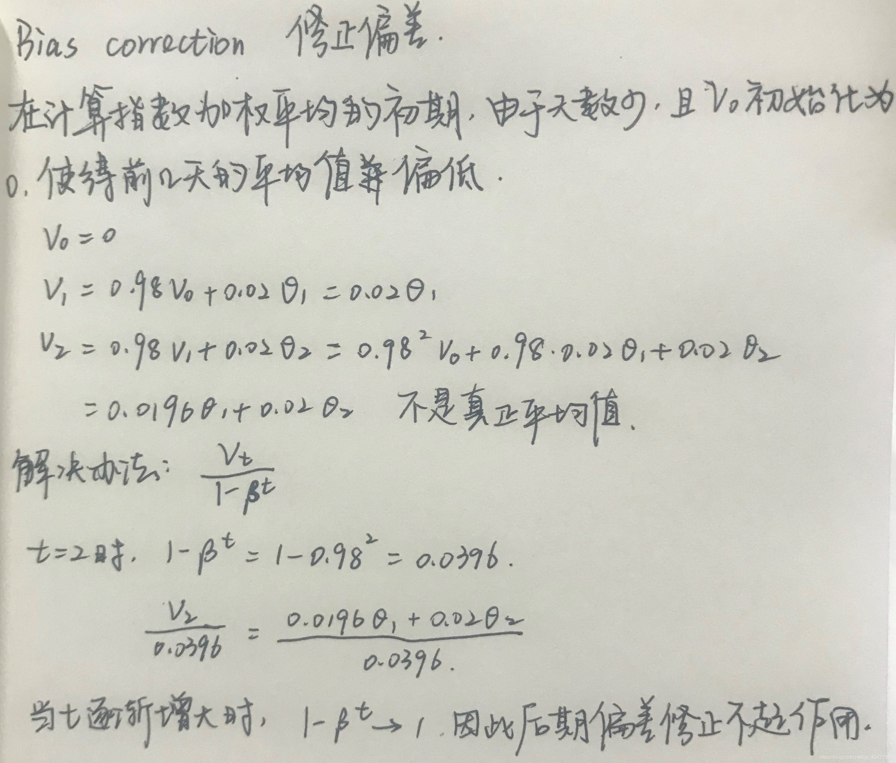
4. 偏差修正

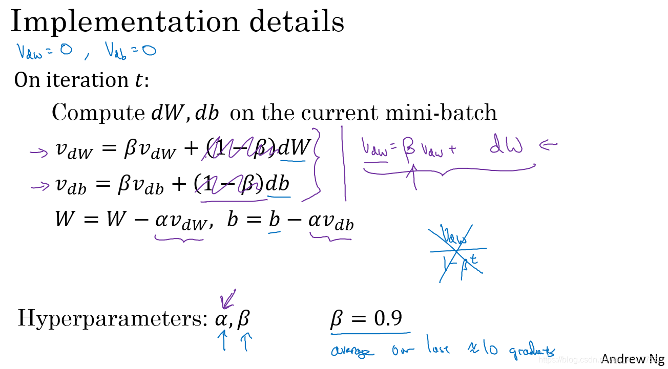
5. Momentum梯度下降法

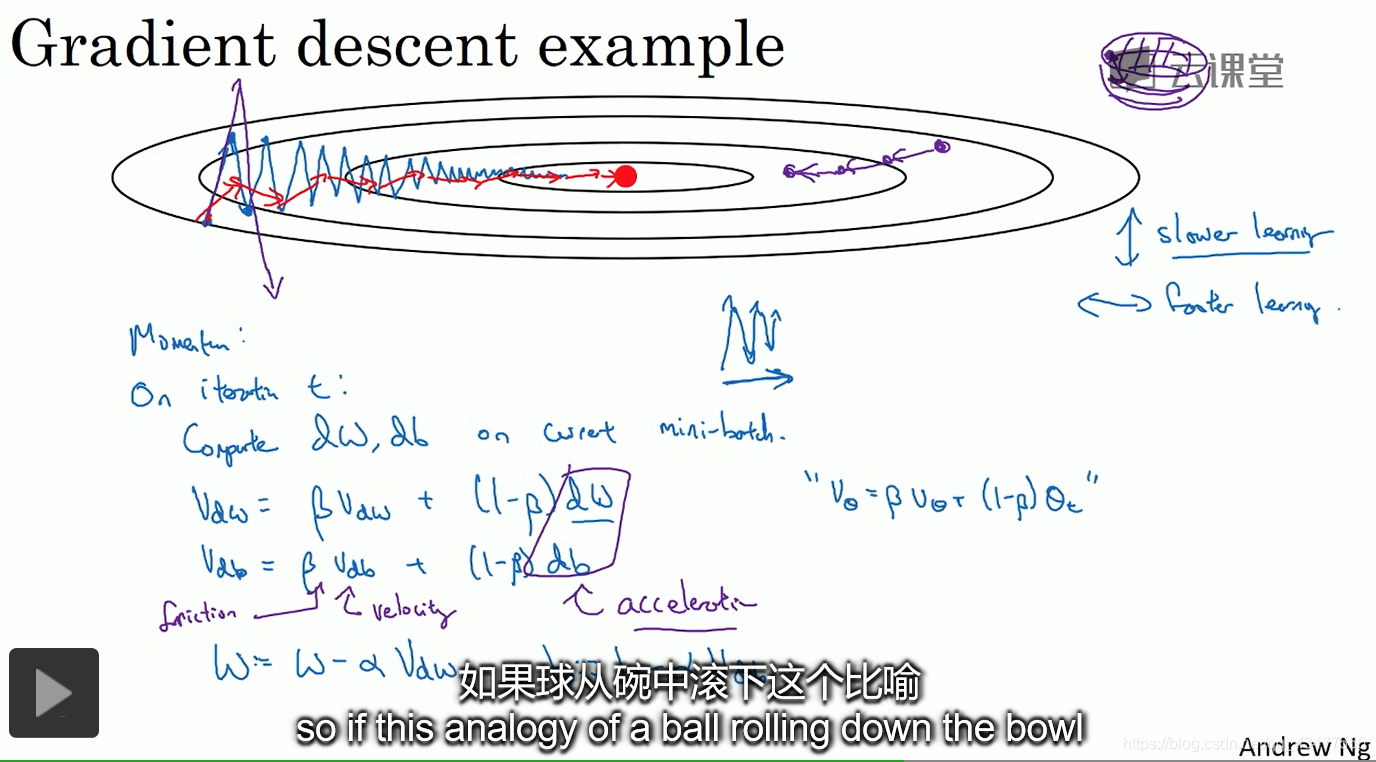
通过指数加权平均，对于纵轴的来回波动可以通过平均相互抵消，从而减缓纵轴的波动，使横轴方向运动更快。
而梯度下降法每次的更新都独立于之前的步骤，因此会随机摆动。
可以将求最小值的过程想象成小球从碗状结构中落到最小值，v相当于速度，β<1相当于摩擦力，防止速度无限增大，dw和db相当于加速度。（v_t=V_0+at）
偏差修正一般不用，因为经过10次迭代后偏差已经消失，无需修正。

6. RMSprop （Root Mean Square prop）
   
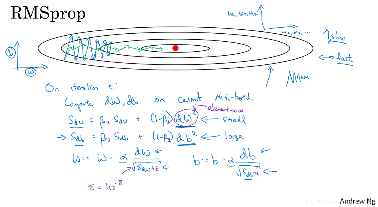
   在垂直方向上，梯度db很大，所以S_db也很大，因此除以一个sqrt(S_db)就可以减轻垂直方向上的摆动，而在水平方向上，梯度dw很小，所以S_dw也很小，因此除以一个较小的数可以加快速度。
   为了防止分母为0，增加一个ε，可以为e-8.
7. Adam(Adaptive moment estimation) optimization algorithm
   是Momentum和RMSprop的结合
   
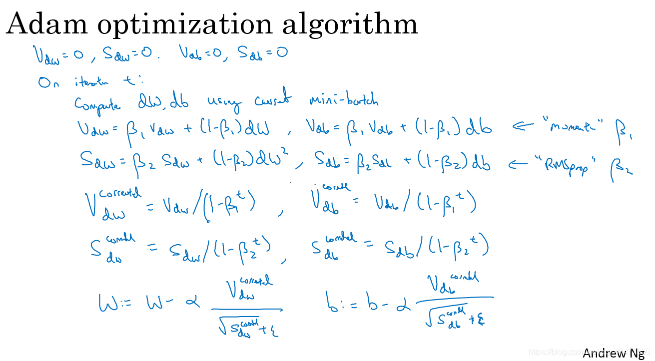
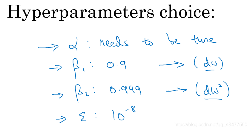
   参数的选择
   

for l in range(L):
   # Moving average of the gradients. Inputs: "v, grads, beta1". Output: "v".
    v["dW" + str(l+1)] = beta1*v["dW"+str(l+1)] + (1-beta1)*grads["dW"+str(l+1)]
    v["db" + str(l+1)] = beta1*v["db"+str(l+1)] + (1-beta1)*grads["db"+str(l+1)]
    # Compute bias-corrected first moment estimate. Inputs: "v, beta1, t". Output: "v_corrected".
    v_corrected["dW" + str(l+1)] = v["dW"+str(l+1)]/(1-np.power(beta1,t))
    v_corrected["db" + str(l+1)] = v["db"+str(l+1)]/(1-np.power(beta1,t))
    # Moving average of the squared gradients. Inputs: "s, grads, beta2". Output: "s".
    s["dW" + str(l+1)] = beta2*s["dW"+str(l+1)]+(1-beta2)*np.power(grads["dW"+str(l+1)],2)
    s["db" + str(l+1)] = beta2*s["db"+str(l+1)]+(1-beta2)*np.power(grads["db"+str(l+1)],2)
    # Compute bias-corrected second raw moment estimate. Inputs: "s, beta2, t". Output: "s_corrected".
    s_corrected["dW" + str(l+1)] = s["dW"+str(l+1)]/(1-np.power(beta2,t))
    s_corrected["db" + str(l+1)] = s["db"+str(l+1)]/(1-np.power(beta2,t))
    # Update parameters. Inputs: "parameters, learning_rate, v_corrected, s_corrected, epsilon". Output: "parameters".
    parameters["W" + str(l+1)] = parameters["W"+str(l+1)] - learning_rate*v_corrected["dW"+str(l+1)]/(np.sqrt(s_corrected["dW"+str(l+1)])+epsilon)
    parameters["b" + str(l+1)] = parameters["b"+str(l+1)] - learning_rate*v_corrected["db"+str(l+1)]/(np.sqrt(s_corrected["db"+str(l+1)])+epsilon)

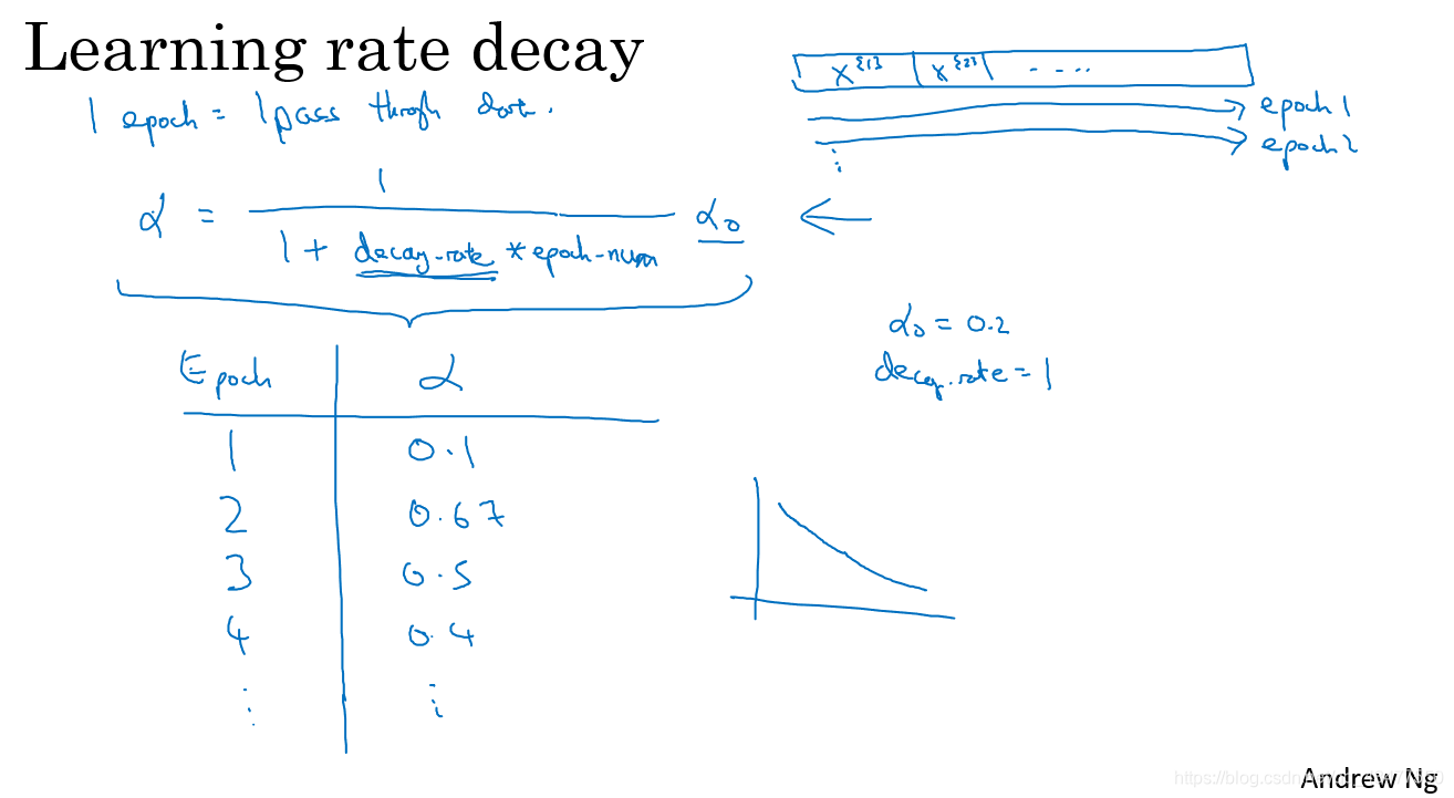
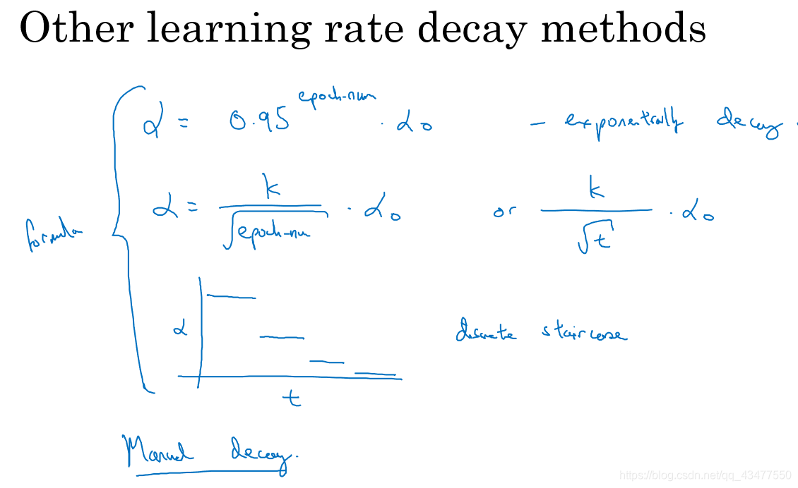
8. learning rate decay 学习率衰减
   
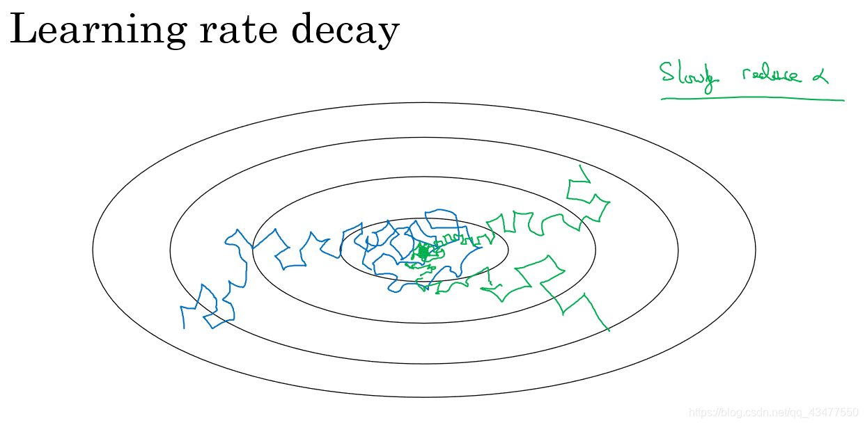
   如果学习率是固定值，mini-match有噪音，可能会导致最后在最优值附近徘徊，不会精确收敛，衰减学习率可以减缓迭代速度，使得更新方向朝着最优值逐渐靠近。
   几种不同的学习率衰减方法：
   
   
9. 平稳值
   
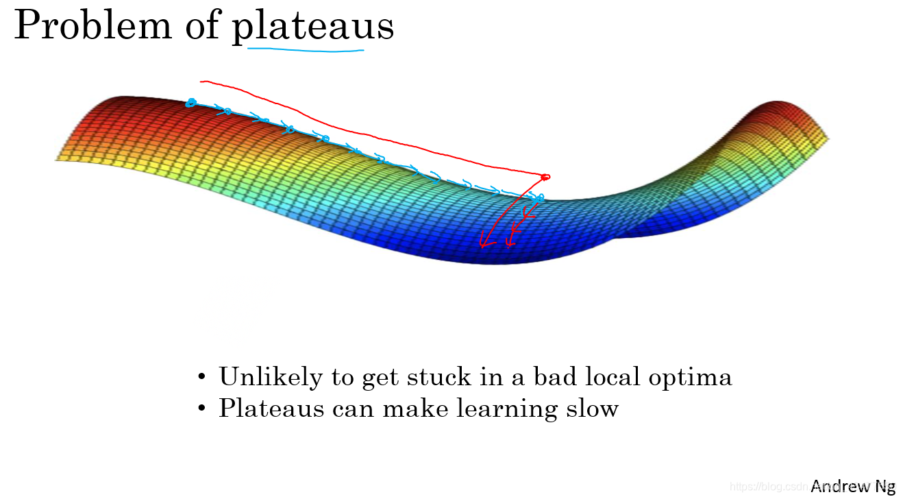
   在一段平稳段中，导数长时间接近于0，会使得学习非常缓慢，这些地方更适用于Momentum和Adam等加速学习算法。

在训练较大神经网络时，不太可能被困在极差的局部最优中，因为参数过多。导数为0的点在鞍点。