MNIST手写数字识别_softmax简单线性回归03

MNIST手写数字识别_softmax简单线性回归

加载数据集，得到训练集和测试集：

mnist = input_data.read_data_sets('D:\pythonProject1\MNIST\MNIST_data',one_hot=True) 
train_X = mnist.train.images
train_Y = mnist.train.labels
test_X = mnist.test.images
test_Y = mnist.test.labels

数据归一化处理：

#数据归一化 min-max 标准化
train_X /= 255
test_X /= 255

数据归一化的主要作用有：
1.去掉量纲，使指标之间具有可比性。
2.将数据限制在一定区间，使运算更为便捷
数据归一化的常用方法：
1.min-max 标准化，使结果映射到0-1之间
x = (x - min) / (max - min)
max为样本数据的最大值，min为样本数据的最小值
2.Z-score 标准化
给予原始数据的均值和标准差进行数据的标准化。处理后的数据符合标准正态分布，即均值为0，标准差为1
x = (x − μ) / σ
μ为样本均值，σ为样本标准差

接下来就可以构建模型啦
深度学习的主要流程为：
1.数据获取（√）
2.数据处理 （√）
3.模型的创建与训练
4.模型测试与评估
5.模型预测

# 构建模型
def create_model():
    #利用Sequential方式构建模型
    model = Sequential()
    model.add(Dense(10))   # 卷积层：提取图像的局部特征  输入为10维的数据？？不确定
    model.add(Activation('softmax')) # 激活函数为softmax
    # 编译模型
   model.compile(loss='categorical_crossentropy',optimizer='adam',metrics=['accuracy'])
   # 设置模型的相关参数：损失函数，优化器，评价指标
    return model
model = create_model()

模型的基础已经构建好了，现在开始训练模型了。

# 模型训练
history = model.fit(train_X,
                    train_Y,
                    batch_size=200, # 每次训练的送入网络中的样本个数
                    epochs=10, # 训练样本送入网络中的次数
                    verbose=2, # 日志输出的复杂度
                    validation_data=(test_X, test_Y))

print(history.history)

使用fit即可训练模型，训练结果保存到history中，我们就可以看到训练的过程啦。

batch_size=200：每次传入200个样本进行训练，一共传入275次，200×275=55000，loss为训练集的损失值，accuracy为训练集的正确率，val_loss为测试值的损失，val_accuracy为测试集的正确率。loss的值越小越好，accuracy的值越大越好。

我们可以绘制一个折线图，方便观察loss和accuracy的变化趋势。

fig = plt.figure()
# 从history中提取我们保存的数据绘制折线图
plt.subplot(2, 1, 1)
plt.plot(history.history['accuracy'])
plt.plot(history.history['val_accuracy'])
plt.title('Model Accuracy')
plt.ylabel('accuracy')
plt.xlabel('epoch')
plt.legend(['train', 'test'], loc='lower right')

plt.subplot(2, 1, 2)
plt.plot(history.history['loss'])
plt.plot(history.history['val_loss'])
plt.title('Model Loss')
plt.ylabel('loss')
plt.xlabel('epoch')
plt.legend(['train', 'test'], loc='upper right')
plt.tight_layout() # 会自动调整子图参数，使之填充整个图像区域

plt.show()

以下5种情况可供参考：
train loss 不断下降，test loss不断下降，说明网络仍在学习;（最好的）
train loss 不断下降，test loss趋于不变，说明网络过拟合;（max pool或者正则化）
train loss 趋于不变，test loss不断下降，说明数据集100%有问题;（检查dataset）
train loss 趋于不变，test loss趋于不变，说明学习遇到瓶颈，需要减小学习率或批量数目;
train loss 不断上升，test loss不断上升，说明网络结构设计不当，训练超参数设置不当，数据集经过清洗等问题。（最不好的情况）

回到我们之前提到过的深度学习的流程，3.模型的创建与训练（√）完成。现在让我们把模型保存起来吧。

# 保存模型
gfile = tf.io.gfile

save_dir = "./MNIST_model/"

if gfile.exists(save_dir):
    gfile.rmtree(save_dir)
gfile.mkdir(save_dir)

model_name = 'mnist_softmax.h5'
model_path = os.path.join(save_dir, model_name)
model.save(model_path)
print('Saved trained model at %s ' % model_path)

训练好的模型一般保存为.h5文件。h5是HDF5文件格式的后缀。h5文件对于存储大量数据而言拥有极大的优势,使用h5文件来存储数据效率高。h5文件是一个将‘group’和‘dataset‘合起来的容器，group像是文件夹，dataset是具体数据，文件，文件夹下可以创建子文件夹，子文件下可以放文件。python 对.h5的操作依赖h5py包，keras可以通过load直接加载.h5文件。
这一部分的代码只需修改保存模型的地址save_dir和模型名称model_name即可。

我们训练好的模型可以直接以.h5文件发给boss，那么boss怎么使用这个模型呢？

# 加载模型 
mnist_model = tf.keras.models.load_model(model_path)

boss需要加载模型，当然model_path的地址是boss保存的地址。

最后我们使用测试集的数据计算出模型的损失和准确率。

# 模型评估
loss_and_metrics = mnist_model.evaluate(test_X, test_Y, verbose=2)

print("Test Loss: {}".format(loss_and_metrics[0]))
print("Test Accuracy: {}".format(loss_and_metrics[1] * 100))

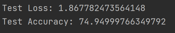
至此，我们看到这个模型的准确率为74.9%，效果不太好，我们试试MLP吧。
完整代码：

import tensorflow as tf
from tensorflow.examples.tutorials.mnist import input_data
import matplotlib.pyplot as plt
import numpy as np
from keras.utils import np_utils
from keras.models import Sequential
from keras.layers import Dense
from keras.layers import Activation
import os

mnist = input_data.read_data_sets('D:\pythonProject1\MNIST\MNIST_data',one_hot=True) # 热编码
train_X = mnist.train.images
train_Y = mnist.train.labels
test_X = mnist.test.images
test_Y = mnist.test.labels

print(train_X.shape, type(train_X))
print(test_X.shape, type(test_X))

# 数据处理
train_X = train_X.astype('float32')
test_X = test_X.astype('float32')

#数据归一化 min-max 标准化
train_X /= 255
test_X /= 255


def creat_model():
    # 定义多层感知机模型
    model = Sequential()
    model.add(Dense(512, input_shape=(784,)))
    model.add(Activation('relu'))

    model.add(Dense(512))
    model.add(Activation('relu'))

    model.add(Dense(10))
    model.add(Activation('softmax'))

    # 编译模型
    model.compile(loss='categorical_crossentropy', optimizer='adam', metrics=['accuracy'])
    return model

model = creat_model()

# 训练模型，保存到history中
history = model.fit(train_X,
                    train_Y,
                    batch_size=128,
                    epochs=10,
                    verbose=2, # 日志输出的复杂度
                    validation_data=(test_X, test_Y))

print(history.history)

# 可视化数据
fig = plt.figure()
plt.subplot(2, 1, 1)
plt.plot(history.history['accuracy'])
plt.plot(history.history['val_accuracy'])
plt.title('Model Accuracy')
plt.ylabel('accuracy')
plt.xlabel('epoch')
plt.legend(['train', 'test'], loc='lower right')

plt.subplot(2, 1, 2)
plt.plot(history.history['loss'])
plt.plot(history.history['val_loss'])
plt.title('Model Loss')
plt.ylabel('loss')
plt.xlabel('epoch')
plt.legend(['train', 'test'], loc='upper right')
plt.tight_layout()

plt.show()

# 保存模型
gfile = tf.io.gfile
save_dir = "./MNIST_model/"
if gfile.exists(save_dir):
    gfile.rmtree(save_dir)
gfile.mkdir(save_dir)

model_name = 'keras_mnist.h5'
model_path = os.path.join(save_dir, model_name)
model.save(model_path)
print('Saved trained model at %s ' % model_path)


# 加载模型
mnist_model = tf.keras.models.load_model(model_path)

# 统计模型在测试上的分类结果
loss_and_metrics = mnist_model.evaluate(test_X, test_Y, verbose=2)

print("Test Loss: {}".format(loss_and_metrics[0]))
print("Test Accuracy: {}".format(loss_and_metrics[1] * 100))