人工智能——衣服分类（大作业必备）

官方网站

大作业系列传送门：💕💕文本分类

导入数据

tf.keras.datasets是一个公开的API可以直接将数据load

import tensorflow as tf
import numpy as np
import matplotlib.pyplot as plt

fashion_mnist = tf.keras.datasets.fashion_mnist
(train_images, train_labels), (test_images, test_labels) = fashion_mnist.load_data()

print("训练集",train_images.shape)
print("训练集标签",train_labels.shape)
print("测试集",test_images.shape)
print("测试集标签 ",len(test_labels))
#训练集(60000, 28, 28)
#训练集标签 (60000,)
#测试集(10000, 28, 28)
#测试集标签 10000

指定名称

#1 T恤/上衣
#2 裤子
#3 套头衫
#4 连衣裙
#5 外套
#6 凉鞋
#7 衬衫
#8 运动鞋
#9 包
#10 短靴

class_names = ['T-shirt/top', 'Trouser', 'Pullover', 'Dress', 'Coat',
               'Sandal', 'Shirt', 'Sneaker', 'Bag', 'Ankle boot']

观察里面图片

#绘图
plt.figure()
plt.imshow(train_images[0])
#给子图添加colorbar（颜色条或渐变色条）
plt.colorbar()
#显示网格线
plt.grid(1)
plt.show()

显示训练集中的前400个图像

plt.figure(figsize=(20,20))
for i in range(400):
    plt.subplot(20,20,i+1)
    #x轴名字
    plt.xticks([i])
    plt.yticks([i])
    plt.grid(False)
    plt.imshow(train_images[i], cmap=plt.cm.binary)
    plt.xlabel(class_names[train_labels[i]])
plt.show()

预处理

归一化（将图像矩阵转化到0-1之间，为了保证精度，经过了运算的图像矩阵I其数据类型会从unit8型变成double型。图像时对double型是认为在0 ~ 1范围内，uint8型时是0~255范围）

train_images = train_images / 255.0

test_images = test_images / 255.0

建立模型

官网模型
模型结构简单易懂

model = tf.keras.Sequential()
#主要的功能就是将(28,28)像素的图像即对应的2维的数组转成28*28=784的一维的数组.
model.add(tf.keras.layers.Flatten(input_shape=(28,28)))
model.add(tf.keras.layers.Dense(64,activation='relu'))
model.add(tf.keras.layers.Dropout(0.5))
model.add(tf.keras.layers.Dense(10,activation='softmax'))
model.summary()

model.compile(optimizer='adam',
              loss=tf.keras.losses.SparseCategoricalCrossentropy(from_logits=True),
              metrics=['accuracy'])
#训练的函数
model.fit(train_images, train_labels, epochs=10)
test_loss, test_acc = model.evaluate(test_images,  test_labels, verbose=2)
print('\nTest accuracy:', test_acc)

模仿VGG16 建立模型

###VGG-16网络结构
from tensorflow.keras import Sequential
from tensorflow.keras.layers import Dense, Dropout, Flatten, BatchNormalization, Conv2D, MaxPool2D
model = Sequential(name = 'Fashion_Model')
# Block1
# 卷积层1
model.add(Conv2D(32, (3, 3), padding = 'same', activation = 'relu',input_shape = (28, 28,1)))
model.add(BatchNormalization())
# 卷积层2
model.add(Conv2D(32, (3, 3), padding = "same", activation = 'relu'))
model.add(BatchNormalization())
model.add(MaxPool2D(pool_size=(2, 2)))

# Block2
# 卷积层3
model.add(Conv2D(64, (3, 3), padding = "same", activation = 'relu'))
model.add(BatchNormalization())
# 卷积层4
model.add(Conv2D(64, (3, 3),padding = "same", activation = 'relu'))
model.add(BatchNormalization())
model.add(MaxPool2D(pool_size=(2, 2)))

# Block3:
# 卷积层5
model.add(Conv2D(128, (3, 3), padding = "same", activation = 'relu'))
model.add(BatchNormalization())
# 卷积层6
model.add(Conv2D(128, (3, 3), padding = "same", activation = 'relu'))
model.add(BatchNormalization())
# 卷积层7
model.add(Conv2D(128, (3, 3), padding = "same",  activation = 'relu'))
model.add(BatchNormalization())
model.add(MaxPool2D(pool_size=(2, 2)))

# Block4
# 卷积层8
model.add(Conv2D(256, (3, 3), padding = "same", activation = 'relu'))
model.add(BatchNormalization())
# # 卷积层9
model.add(Conv2D(256, (3, 3), padding = "same", activation = 'relu'))
model.add(BatchNormalization())
## 卷积层10
model.add(Conv2D(256, (3, 3), padding = "same", activation = 'relu'))
model.add(BatchNormalization())
model.add(MaxPool2D(pool_size=(2, 2)))

# Block5
# 卷积层11
model.add(Conv2D(512, (3, 3), padding = "same", activation = 'relu'))
model.add(BatchNormalization())
# # 卷积层12
model.add(Conv2D(512, (3, 3), padding = "same", activation = 'relu'))
model.add(BatchNormalization())
## 卷积层13
#model.add(Conv2D(512, (3, 3),padding = "same", activation = 'relu'))
#model.add(BatchNormalization())
#model.add(MaxPool2D(pool_size=(2, 2)))
# 全连接层FC：第14层
model.add(Flatten())
model.add(Dense(64, activation = 'relu'))
model.add(BatchNormalization())
model.add(Dropout(0.5))

# Block6
# 全连接层FC：第15层
model.add(Dense(64, activation = 'relu'))
model.add(BatchNormalization())
model.add(Dropout(0.5))

# Block7
# 全连接层FC：第16层，Softmax分类        
model.add(Dense(10, activation = 'softmax'))
          
# 模型结构
model.summary()

编译模型

Adam方法，此处可选。
损失函数是SparseCategoricalCrossentropy

model.compile(optimizer='adam',
              loss=tf.keras.losses.SparseCategoricalCrossentropy(from_logits=True),
              metrics=['accuracy'])

开始训练

fit函数自行查阅，这里只返回loss和- accuracy

train_images=train_images.reshape(60000,28,28,1)
hist = model.fit(train_images, train_labels, epochs=10)

绘制曲线

def training_vis(hist):
    loss = hist.history['loss']
    acc = hist.history['accuracy']  # new version => hist.history['accuracy'] 
    # make a figure
    fig = plt.figure(figsize=(10,4))
    # subplot loss
    ax1 = fig.add_subplot(121)
    ax1.plot(loss,label='train_loss')
    ax1.set_xlabel('Epochs')
    ax1.set_ylabel('Loss')
    ax1.set_title('Loss on Training and Validation Data')
    ax1.legend()
    # subplot acc
    ax2 = fig.add_subplot(122)
    ax2.plot(acc,label='train_acc')
    ax2.set_xlabel('Epochs')
    ax2.set_ylabel('Accuracy')
    ax2.set_title('Accuracy  on Training and Validation Data')
    ax2.legend()
    plt.tight_layout()
training_vis(hist)

模型评估

转置后使用执行函数model.evaluate直接得到最后的测试集准确率。

test_images=test_images.reshape(10000,28,28,1)
test_loss, test_acc = model.evaluate(test_images,  test_labels, verbose=1)

print('\nTest accuracy:', test_acc)

图形测试定义

probability_model = tf.keras.Sequential([model, 
                                         tf.keras.layers.Softmax()])
predictions = probability_model.predict(test_images)

#显示图片，正确的标签是蓝色，错误的是红色
def plot_image(i, predictions_array, true_label, img):
  true_label, img = true_label[i], img[i]
  plt.grid(False)
  plt.xticks([])
  plt.yticks([])

  plt.imshow(img, cmap=plt.cm.binary)

  predicted_label = np.argmax(predictions_array)
  if predicted_label == true_label:
    color = 'blue'
  else:
    color = 'red'

  plt.xlabel("{} {:2.0f}% ({})".format(class_names[predicted_label],
                                100*np.max(predictions_array),
                                class_names[true_label]),
                                color=color)
#定义一个函数来显示图片每个概率的柱状图，正确的是蓝色，错误的是红色
def plot_value_array(i, predictions_array, true_label):
  true_label = true_label[i]
  plt.grid(False)
  plt.xticks(range(10))
  plt.yticks([])
  thisplot = plt.bar(range(10), predictions_array, color="#777777")
  plt.ylim([0, 1])
  predicted_label = np.argmax(predictions_array)

  thisplot[predicted_label].set_color('red')
  thisplot[true_label].set_color('blue')

验证结果

预测多张结果

num_rows = 5
num_cols = 3
num_images = num_rows*num_cols
plt.figure(figsize=(2*2*num_cols, 2*num_rows))
for i in range(num_images):
  plt.subplot(num_rows, 2*num_cols, 2*i+1)
  plot_image(i, predictions[i], test_labels, p)
  plt.subplot(num_rows, 2*num_cols, 2*i+2)
  plot_value_array(i, predictions[i], test_labels)
plt.tight_layout()
plt.show()

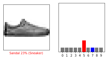
预测单张结果

i = 12
plt.figure(figsize=(6,3))
plt.subplot(1,2,1)
plot_image(i, predictions[i], test_labels, test_images)
plt.subplot(1,2,2)
plot_value_array(i, predictions[i],  test_labels)
plt.show()

总结：用了VGG结构准确率确实提高不少，就是需要时间过长，仅以此学习熟悉结构。