快速幂、矩阵快速幂

快速幂

所谓快速幂，就是用来快速求取$a^n$的算法，当$n$不大时，或者需要求取的次数不多时，我们可以直接进行$n$次遍历求取即可，当$n$的很大或者需要多次求取时，我们有一种更为快速的算法来求解，有多快？—$O(logn)$
$$\begin{gathered} 我们考虑a^n，分解n，即将n转化为二进制形式，假设n=27 \\ 则，a^{27}=a^{(11011{)}_{2进制}}=a^{(10000{)}_2}\ast a^{(1000{)}_2}\ast a^{(10{)}_2}\ast a^{(1{)}_2} \\ =a^{16}\ast a^8\ast a^2\ast a^1=a^{27}.......(对n进行二进制分解) \end{gathered}$$
那么我们根据上面的分解步骤就可以的到，
当前n的二进制位值第x为1时，只需要乘上$a^{2^x}$即可，并且每次a*a，就能得到下一个位置x+1的$a^{2^{x+1}}$。
我们直接来看代码
例题:acwing875. 快速幂
代码如下：

#include<cstdio>
#include<iostream>
#include<algorithm>
#include<cstring>
using namespace std;
typedef long long ll;
int ks(int a,int b,int p){
    int res=1;
    while(b){
        if(b&1) res=(ll)res*a%p;
        a=(ll)a*a%p;
        b>>=1;
    }
    return res%p;
}
int main(){
    int t,a,b,p;;
    cin>>t;
    while(t--){
        scanf("%d%d%d",&a,&b,&p);
        printf("%d\n",ks(a,b,p));
    }
    return 0;
}

矩阵快速幂

矩阵快速幂=快速幂+矩阵乘法

首先，我们先了解一下矩阵乘法的规则：

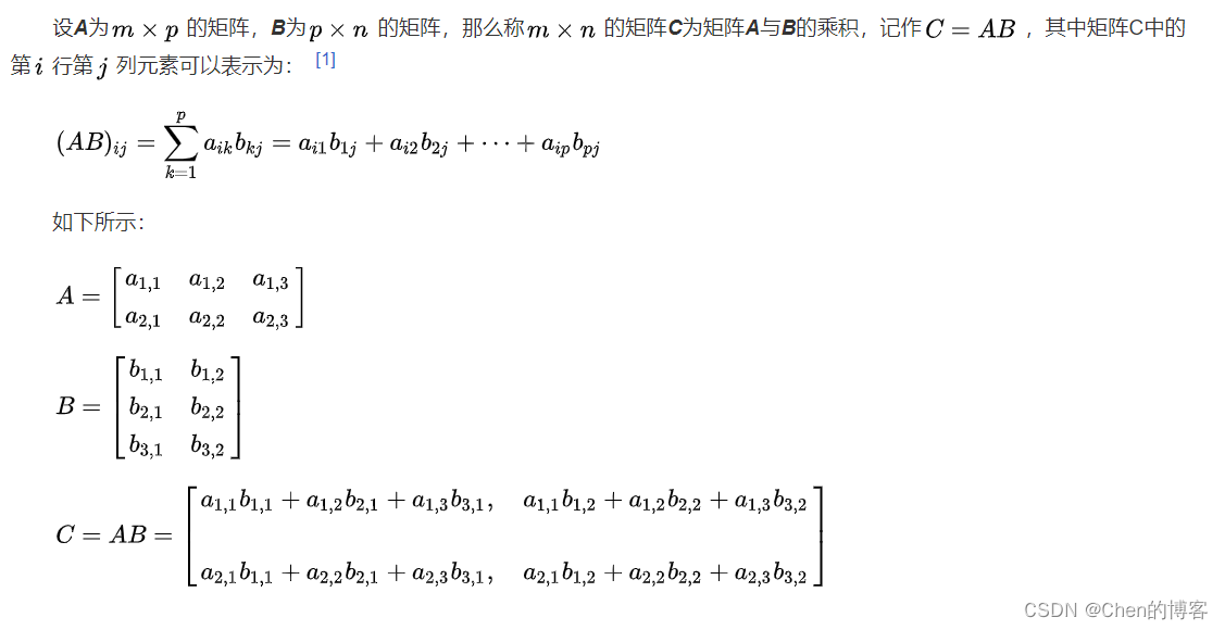
$$\begin{gathered} 矩阵A要想与矩阵B相乘，那么矩阵A的列数就得等于矩阵B的行数 \\ 即，C_{a\times b}=A_{a\times p}\times B_{p\times b} \\ 所得新矩阵C的行数等于矩阵A的行数，列数等于矩阵B的列数 \end{gathered}$$
由斐波那契数列来来引出矩阵快速幂
$$\begin{gathered} f[n]=\{\begin{array}{l}f[n-1]+f[n-2],n>1\\ f[1]=1\\ f[0]=0\end{array} \\ 可以写成\left[\begin{array}{cc}f[n]& 0\\ f[n-1]& 0\end{array}\right]=\left[\begin{array}{cc}1& 1\\ 1& 0\end{array}\right]\times \left[\begin{array}{cc}f[n-1]& 0\\ f[n-2]& 0\end{array}\right]={\left[\begin{array}{cc}1& 1\\ 1& 0\end{array}\right]}^2\times \left[\begin{array}{cc}f[n-2]& 0\\ f[n-3]& 0\end{array}\right] \\ 依次类推可得： \\ \left[\begin{array}{cc}f[n]& 0\\ f[n-1]& 0\end{array}\right]={\left[\begin{array}{cc}1& 1\\ 1& 0\end{array}\right]}^{n-1}\times \left[\begin{array}{cc}f[1]& 0\\ f[0]& 0\end{array}\right] \end{gathered}$$
也就是说，我们只需要算出${\left[\begin{array}{cc}1& 1\\ 1& 0\end{array}\right]}^{n-1}$即可求出$\left[\begin{array}{cc}f[n]& 0\\ f[n-1]& 0\end{array}\right]$，而${\left[\begin{array}{cc}1& 1\\ 1& 0\end{array}\right]}^{n-1}$我们可以用快速幂的思想在$O(logn)$的时间复杂度内求出。
例题：acwing205. 斐波那契
代码如下：

#include<cstdio>
#include<iostream>
#include<algorithm>
#include<cstring>
using namespace std;
typedef long long ll;
const int P=10000; 

struct node{
    int data[5][5];
};
node mul(node a,node b){//矩阵乘法
    node res;
    memset(res.data,0,sizeof res.data);
    for(int i=1;i<=2;i++)
        for(int j=1;j<=2;j++)
            for(int k=1;k<=2;k++)
                res.data[i][j]=(res.data[i][j]+(ll)a.data[i][k]*b.data[k][j]%P)%P;
    return res;
}

node ks(node a,int b){//快速幂
    node res;
    memset(res.data,0,sizeof res.data);
    for(int i=1;i<=2;i++) res.data[i][i]=1;
    while(b){
        if(b&1) res=mul(res,a);
        b>>=1;
        a=mul(a,a);
    }
    return res;
}

int main(){
    int n;
    while(scanf("%d",&n)&&n!=-1){
        if(!n){
            printf("0\n");
            continue;
        }
        node f,base;
        f.data[1][1]=1;f.data[1][2]=0;//初始斐波那契数列
        f.data[2][1]=0;f.data[2][2]=0;
        
        base.data[1][1]=1;base.data[1][2]=1;//构建矩阵
        base.data[2][1]=1;base.data[2][2]=0;
        
        node ant=ks(base,n-1);
        
        node res=mul(ant,f);
        
        cout<<res.data[1][1]<<endl;
        
    }
    return 0;
}

斐波那契数列差不多是最简单的矩阵快速幂的应用，矩阵快速幂的难点在于如何构建一个矩阵，使其能够满足递推式。