机器学习-逻辑回归(吴恩达课后作业)

1.1 逻辑回归

在我理解中就是用来进行分类，虽然叫回归，实际上是分类模型，常用的是二分类问题。

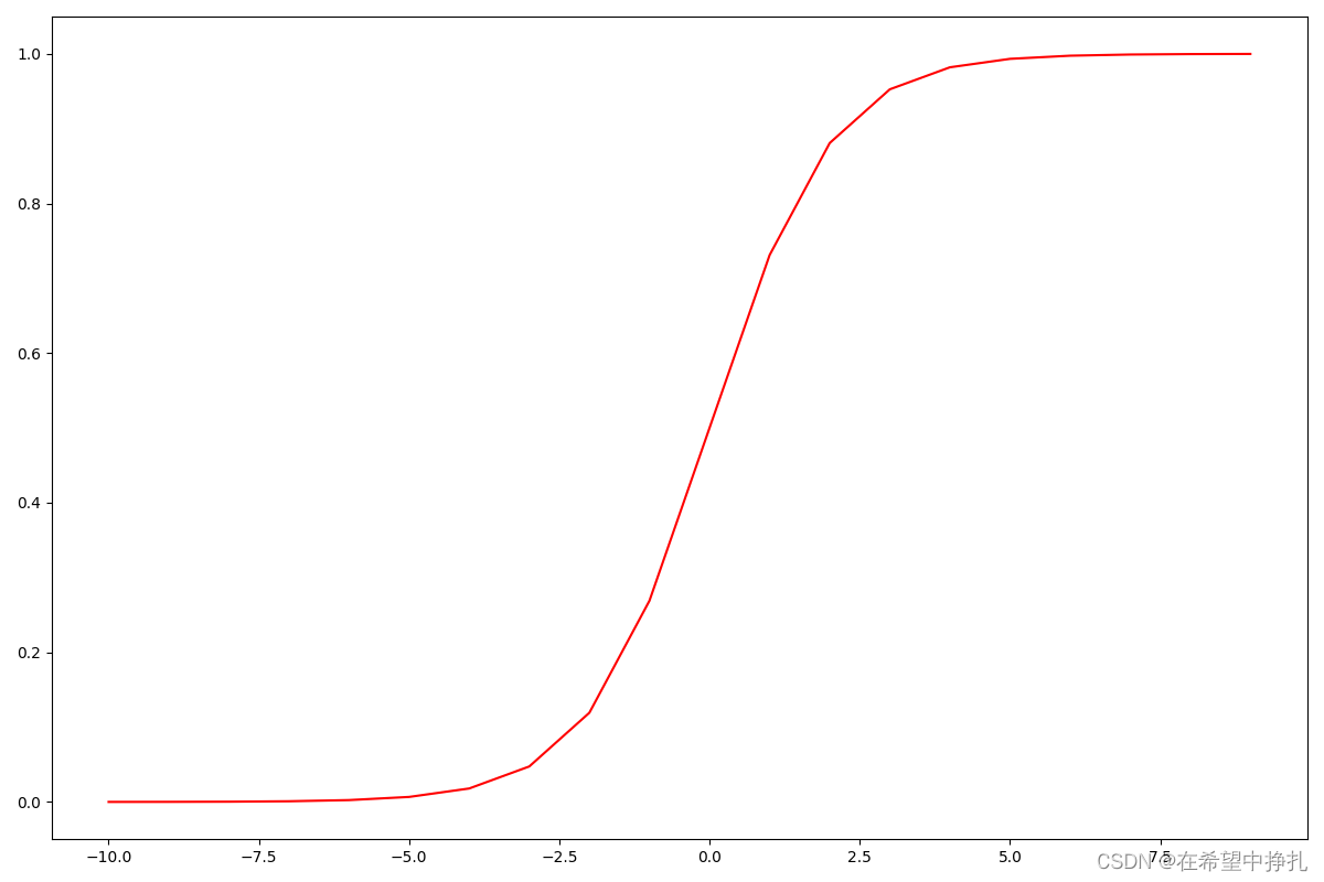
1.2 sigmoid函数

def sigmoid(z):
    return 1.0 / (1 + np.exp(-z))

1.3 代价函数

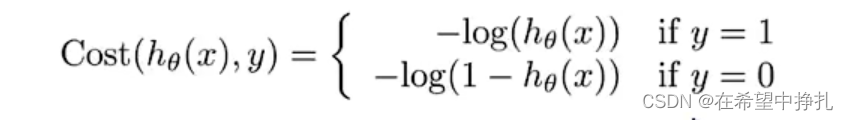
当时理解了很久，可以把这两个函数的图画出来可以更好的理解，当y=1的时候，可以想象成如果点距离决策边界越远(也就是我们找到的分界)，其值就越大，在sigmoid函数里，z在趋于无穷时，sigmoid越趋近于1，log之后为0。即很好的把这个点分界出来了，所产生的代价就越小，相反没有被很好的隔离开会产生很大代价。y=0时也是这样，越趋于负无穷时，也就是决策边界下方的点距离的越远时候，其sigmoid函数越区域0，这是的代价应该是最小的，所以在代价函数中y=0，为-log(1-h(x)), 需要用1减。

1.4 梯度下降

这里使用用SciPy的“optimize”命名空间来做同样的事情。

res = opt.fmin_tnc(func=Cost, x0=theta, fprime=gradient, args=(X,y))

1.5Code

# -*- coding: utf-8 -*-
# @Time : 2022/5/14 17:56
# @Author : Yao Guoliang
import numpy as np
import matplotlib.pyplot as plt
import pandas as pd
import scipy.optimize as opt

def showData(positive, negative):
    fig, ax = plt.subplots(figsize=(12,8))
    ax.scatter(positive['exam1'], positive['exam2'], s=50, c='b', marker='o', label='Admitted')
    ax.scatter(negative['exam1'], negative['exam2'], s=50, c='r', marker='x', label='Not Admitted')
    ax.legend()
    ax.set_xlabel('exam1 Score')
    ax.set_ylabel('exam2 Score')
    plt.show()

def sigmoid(z):
    return 1.0 / (1 + np.exp(-z))

# sigmoid Test
def sigmoidTest():
    nums = np.arange(-10, 10, 1)
    fig, ax = plt.subplots(figsize=(12,8))
    ax.plot(nums, sigmoid(nums), 'r')
    plt.show()

# 计算损失函数
def Cost(theta, X, y):
    theta = np.matrix(theta)
    X = np.matrix(X)
    y = np.matrix(y)
    first = np.multiply(-y, np.log(sigmoid(X * theta.T)))
    second = np.multiply((1 - y), np.log(1 - sigmoid(X * theta.T)))
    return np.sum(first - second) / (len(X))

# 梯度下降
def gradient(theta, X, y):
    theta = np.matrix(theta)
    X = np.matrix(X)
    y = np.matrix(y)
    parameters = int(theta.ravel().shape[1])
    # print(parameters)   3
    grad = np.zeros(parameters)
    error = sigmoid(X * theta.T) - y
    # print(error)
    for i in range(parameters):
        term = np.multiply(error, X[:, i])
        grad[i] = np.sum(term) / len(X)
    return grad

def predict(theta, X):
    probability = sigmoid(X * theta.T)
    return [1 if x >= 0.5 else 0 for x in probability]

if __name__ == '__main__':
    data = pd.read_csv('./data/ex2data1.txt', names=['exam1', 'exam2', 'Admitted'])
    # 查看数据
    # print(data.head())
    # print(data.describe())
    positive = data[data['Admitted'].isin([1])]
    negative = data[data['Admitted'].isin([0])]
    # showData(positive, negative)
    sigmoidTest()
    data.insert(0, 'Ones', 1)
    # print(data)
    clos = data.shape[1]
    X = data.iloc[:, :clos - 1]
    y = data.iloc[:, clos - 1:clos]
    X = np.array(X.values)
    y = np.array(y.values)
    theta = np.zeros(X.shape[1])
    # print(X.shape, y.shape, theta)
    inCost = Cost(theta, X, y)
    print(inCost)
    grad = gradient(theta ,X, y)
    # print(grad)
    res = opt.fmin_tnc(func=Cost, x0=theta, fprime=gradient, args=(X,y))
    print(res)
    print(Cost(res[0], X, y))
    theta_min = np.matrix(res[0])
    predicts = predict(theta_min, X)

    ans = 0
    for i in range(len(predicts)):
        if(predicts[i] == y[i]) :
            ans += 1
    accuracy = ans / len(X)
    # 准确率
    print(accuracy)

    x1 = np.arange(130, step=0.1)
    x2 = -(res[0][0] + x1 * res[0][1]) / res[0][2]
    # print(x2)
    fig, ax = plt.subplots(figsize=(8, 6))
    ax.scatter(positive['exam1'], positive['exam2'], c='orange', label='Admitted')
    ax.scatter(negative['exam1'], negative['exam2'], c='b', marker='*', label='Not Admitted')
    ax.plot(x1,x2)
    ax.set_xlim(0, 130)
    ax.set_ylim(0, 130)
    ax.set_xlabel('x1')
    ax.set_ylabel('x2')
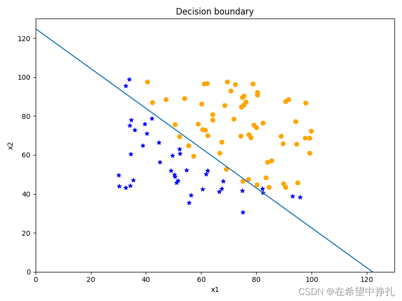
    ax.set_title('Decision boundary')
    plt.show()

1.6结果