Andrew NG机器学习逻辑回归编程作业

Exercise 2：Logistic Regression—实现一个逻辑回归
问题描述：用逻辑回归根据学生的考试成绩来判断该学生是否可以入学。

这里的训练数据(training instance)是学生的两次考试成绩，以及TA是否能够入学的决定（y=0表示成绩不合格，不予录取；y=1表示录取）

因此，需要根据trainging set 训练出一个classification model。然后，拿着这个classification model 来评估新学生能否入学。

训练数据的成绩样例如下：第一列表示第一次考试成绩，第二列表示第二次考试成绩，第三列表示入学结果（0–不能入学，1–可以入学）

34.62365962451697, 78.0246928153624,  0
30.28671076822607, 43.89499752400101, 0
35.84740876993872, 72.90219802708364, 0
60.18259938620976, 86.30855209546826, 1
...               ...

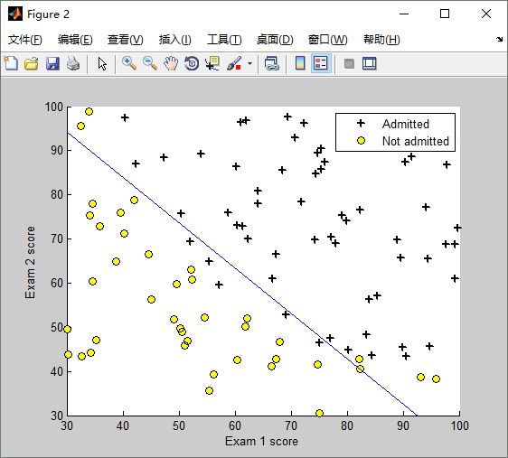
训练数据图形表示 如下：橫坐标是第一次考试的成绩，纵坐标是第二次考试的成绩，右上角的 + 表示允许入学，圆圈表示不允许入学。（分数决定命运，太悲惨了！）

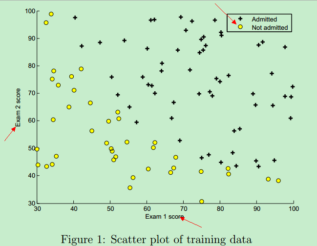
该训练数据的图形 可以通过Matlab plotData函数画出来,它调用Matlab中的plot函数和find函数，Matlab代码实现如下：
0. Visualizing the data
Matlab将文本文件中的训练数据加载到 矩阵X 和 向量 y 中

%Initialization
clear all; close all; clc

data = csvread('ex2data1.txt');
X = data(:, [1, 2]); y = data(:, 3);
%X读取的是第一列和第二列的所有数据
%y读取的是第三列的所有数据

录取的点用+表示，未录取的点用圆圈o表示。plotData函数的框架如下：

% ==================== Part 1: Plotting ====================

fprintf(['Plotting data with + indicating (y = 1) examples and o ' ...
         'indicating (y = 0) examples.\n']);
function plotData(X, y)
    figure; hold on;
%====================== YOUR CODE HERE ======================
    xlabel('Exam 1 score')
    ylabel('Exam 2 score')
    legend('Admitted', 'Not admitted')
    hold off;
end

加载完数据之后，执行以下代码（调用自定义的plotData函数），将图形画出来：

function plotData(X, y)
figure; hold on;

% ====================== YOUR CODE HERE ======================


pos = find(y == 1);
neg = find(y == 0);

plot(X(pos,1),X(pos,2),'k+','Linewidth',2,'MarkerSize',7);
plot(X(neg,1),X(neg,2),'ko','MarkerFaceColor','y','MarkerSize',7);

注释：
1.pos = find(y == 1）
找到y等于1的，数据的行数
neg = find(y == 0);
找到y等于0的，数据的行数
X(pos,1)表示X中，第pos行，第一列数据
X(pos,2)表示X中，第pos行，第二列数据
下面类似，不在赘述
2.plot(X(pos,1),X(pos,2),’k+’,’Linewidth’,2,’MarkerSize’,7);
表示。画出，横坐标等于X(pos,1)纵坐标等于X(pos,2)的点。用+号表示，线宽为2，大小为7
下面类似

---

图形画出来之后，对训练数据就有了一个大体的可视化的认识了。接下来就要实现 模型了，这里需要训练一个逻辑回归模型。

1. sigmoid function
要求实现如下函数，实现时z是向量，要对每个元素都做计算。

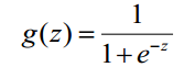
function g = sigmoid(z)
    g = zeros(size(z));设置初值
    g = 1 ./ (1 + exp(-z));
    %‘点除’ 表示 1 除以矩阵(向量)中的每一个元素
end

1. Cost function and gradient
   先来看一下计算前的准备工作

%% ============ Part 2: Compute Cost and Gradient ============

[m, n] = size(X);

X = [ones(m, 1) X];%向量化的常规套路，增加一行X0

initial_theta = zeros(n + 1, 1);%重置初值

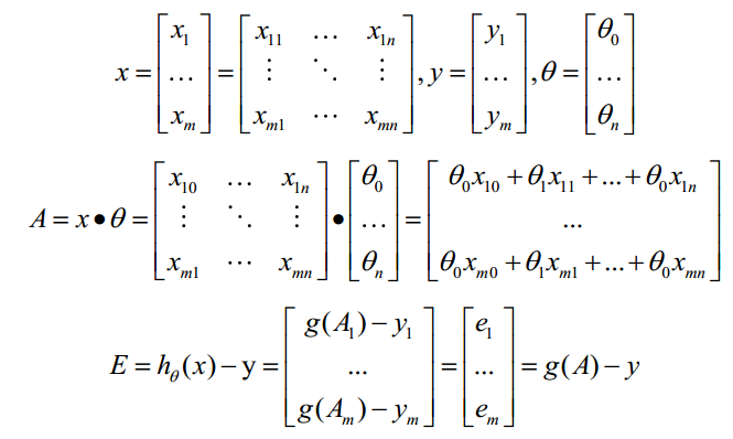
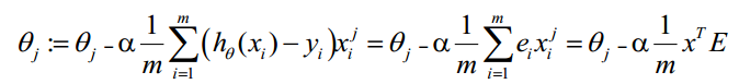
[cost, grad] = costFunction(initial_theta, X, y);

X是个矩阵，它每列表示一个特征，每行表示一个实例。theta是n+1个元素的列向量。y是m个元素的结果向量。

代价函数公式

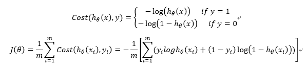
可以先用一个变量hx求出h(x)，利用1中的函数

hx = sigmoid(X * theta);

求和号中每一项对应一行，可以使用向量化的方法计算，最后用sum求和。

J = (-1/m) * sum(y .* log(hx) + (1-y) .* log(1 - hx));

梯度的计算公式


代价函数costFunction（）的定义如下

function [J, grad] = costFunction(theta, X, y)
    m = length(y); % number of training examples
    grad = zeros(size(theta));
    hx = sigmoid(X * theta);
    J = (-1/m) * sum(y .* log(hx) + (1-y) .* log(1 - hx));

    n = length(theta);
    for j = 1 : n
        grad(j) = sum((hx - y) .* X(:, j)) / m;
         % X 为 training set 中的 feature variables, y 为training instance(训练样本的结果)结果，相当于对j
    end
end

通过调用costfunction.m文件中定义的coustFunction函数，从而运行梯度下降算法找到使代价函数J(theta)最小化的 逻辑回归模型参数theta。调用costFunction函数的代码如下：
3. fminunc

%  Set options for fminunc
options = optimset('GradObj', 'on', 'MaxIter', 400);
 %  Run fminunc to obtain the optimal theta
 %  This function will return theta and the cost 
[theta, cost] = ...
    fminunc(@(t)(costFunction(t, X, y)), initial_theta, options);
 % Plot Boundary
plotDecisionBoundary(theta, X, y);

注释：
1.fminunc中的@(t)(costFunction(t, X, y))是为了把函数costFunction转换为只接受一个参数t的函数。

2.从上面代码的最后一行可以看出，我们是通过 fminunc 调用 costFunction函数，来求得 theta的，而不是自己使用 Gradient descent 在for 循环求导来计算 theta。for循环中求导计算theta，
既然已经通过Gradient descent算法求得了theta，将theta代入到假设函数中，就得到了 logistic regression model.

调用plotDecisionBoundary函数画出点和决策边界，其中相关的代码如下（两个参数的情况）

if size(X, 2) <= 3
    % Only need 2 points to define a line, so choose two endpoints
    plot_x = [min(X(:,2))-2,  max(X(:,2))+2];

    % Calculate the decision boundary line
    plot_y = (-1./theta(3)).*(theta(2).*plot_x + theta(1));

    % Plot, and adjust axes for better viewing
    plot(plot_x, plot_y)

    % Legend, specific for the exercise
    legend('Admitted', 'Not admitted', 'Decision Boundary')
    axis([30, 100, 30, 100])

？？？？？？？？？？以上边界函数代码看不懂，先放弃，以后再看，先往下进行。

ex2的第104行是不需要的，因为在上面函数里已经添加了图示。在运行legend(‘Admitted’, ‘Not admitted’)反而会覆盖掉分界线的图示。
将theta代入到假设函数中，就得到了 logistic regression model，用图形表示如下：

4. predict 模型的评估（Evaluating logistic regression）

那如何估计，求得的逻辑回归模型是好还是坏呢？预测效果怎么样？因此，就需要拿一组数据测试一下，测试代码如下：

%% ============== Part 4: Predict and Accuracies ==============

prob = sigmoid([1 45 85] * theta); %这是一组测试数据，第一次考试成绩为45，第二次成绩为85
fprintf(['For a student with scores 45 and 85, we predict an admission ' ...
         'probability of %f\n\n'], prob);

% Compute accuracy on our training set
p = predict(theta, X);% 调用predict函数测试模型

fprintf('Train Accuracy: %f\n', mean(double(p == y)) * 100);

fprintf('\nProgram paused. Press enter to continue.\n');
pause;

模型的测试结果如下：

For a student with scores 45 and 85, we predict an admission probability of 0.774323

Train Accuracy: 89.000000

那predict函数是如何实现的呢？predict.m 如下：

function p = predict(theta, X)

m = size(X, 1); % Number of training examples

p = zeros(m, 1);

% ====================== YOUR CODE HERE ======================
% Instructions: Complete the following code to make predictions using
%               your learned logistic regression parameters. 
%               You should set p to a vector of 0's and 1's
%
p = X*theta >= 0;

% =========================================================

end

备注：double(y)表示将参数y转为双精度浮搜索点类型.mean(A)表示求A的平均值
非常简单，只有一行代码：p = X * theta >= 0，原理如下：

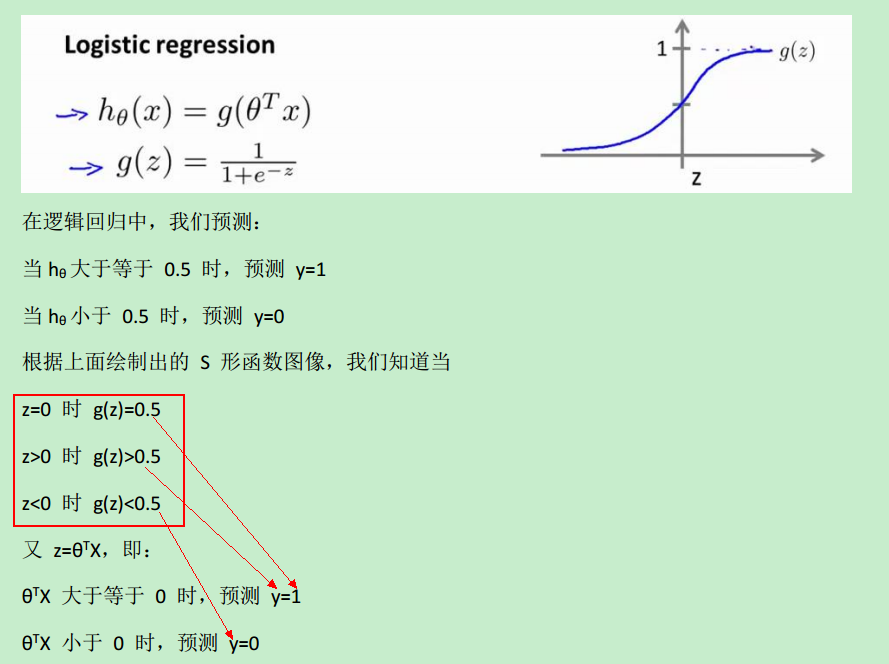
当h(x)>=0.5时，预测y==1，而h(x)>=0.5 等价于 z>=0

---

Regularization
为什么需要正则化？正则化就是为了解决过拟合问题(overfitting problem)。那什么又是过拟合问题呢？

一般而言，当模型的特征(feature variables)非常多，而训练的样本数目(training set)又比较少的时候，训练得到的假设函数(hypothesis function)能够非常好地匹配training set中的数据，此时的代价函数几乎为0。下图中最右边的那个模型 就是一个过拟合的模型。

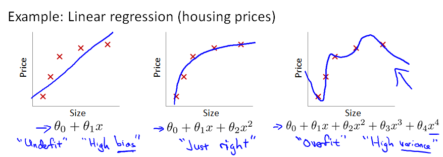
**所谓过拟合，从图形上看就是：假设函数曲线完美地通过中样本中的每一个点。也许有人会说：这不正是最完美的模型吗？它完美地匹配了traing set中的每一个样本呀！

过拟合模型不好的原因是：尽管它能完美匹配traing set中的每一个样本，但它不能很好地对未知的 (新样本实例)input instance 进行预测呀！通俗地讲，就是过拟合模型的预测能力差。

因此，正则化(regularization)就出马了。

前面提到，正是因为 feature variable非常多，导致 hypothesis function 的幂次很高，hypothesis function变得很复杂(弯弯曲曲的)，从而通过穿过每一个样本点(完美匹配每个样本)。如果添加一个”正则化项”，减少 高幂次的特征变量的影响，那 hypothesis function不就变得平滑了吗？

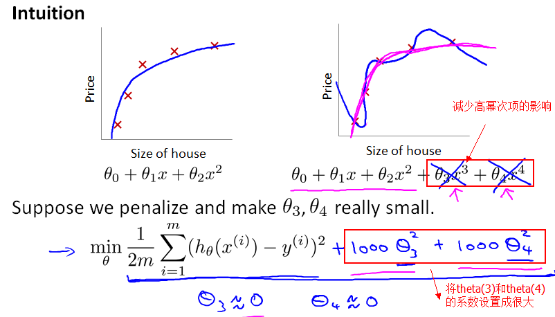
正如前面提到，梯度下降算法的目标是最小化cost function，而现在把 theta(3) 和 theta(4)的系数设置为1000，设得很大，求偏导数时，相应地得到的theta(3) 和 theta(4) 就都约等于0了。

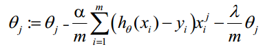
更一般地，我们对每一个theta(j)，j>=1，进行正则化，就得到了一个如下的代价函数：其中的 lambda(λ)就称为正则化参数(regularization parameter)

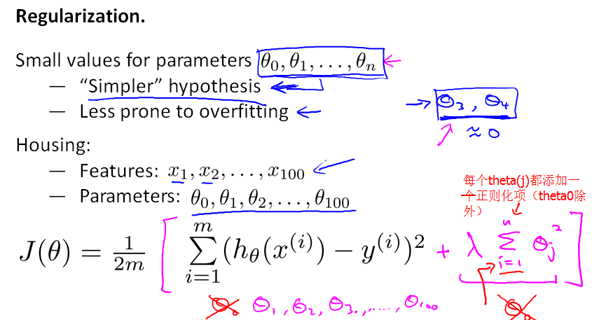
从上面的J(theta)可以看出：如果lambda(λ)=0，则表示没有使用正则化；如果lambda(λ)过大，使得模型的各个参数都变得很小，导致h(x)=theta(0)，从而造成欠拟合；如果lambda(λ)很小，则未充分起到正则化的效果。因此，lambda(λ)的值要合适。

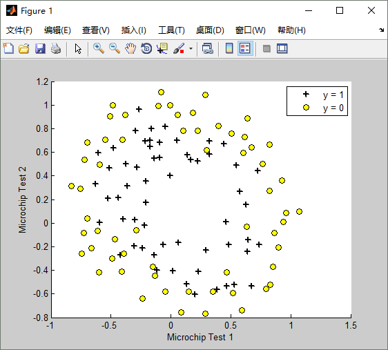
最后，我们来看一个实际的过拟合的示例，原始的训练数据如下图：

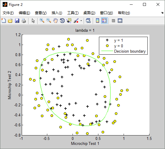
lambda(λ)==1时，训练出来的模型（hypothesis function）如下：Train Accuracy: 83.050847

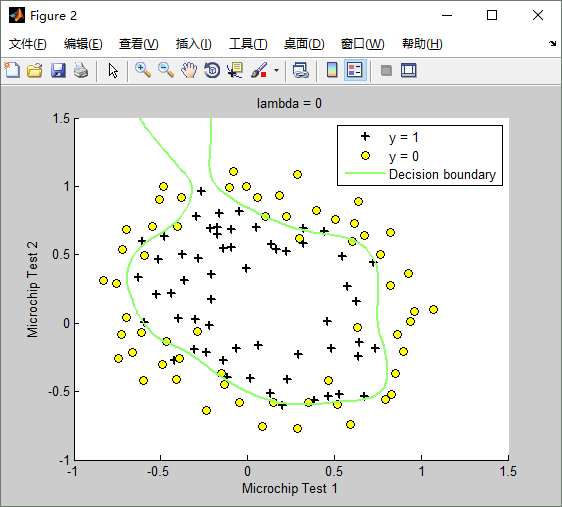
lambda(λ)==0时，不使用正则化，训练出来的模型（hypothesis function）如下：Train Accuracy: 87.288136

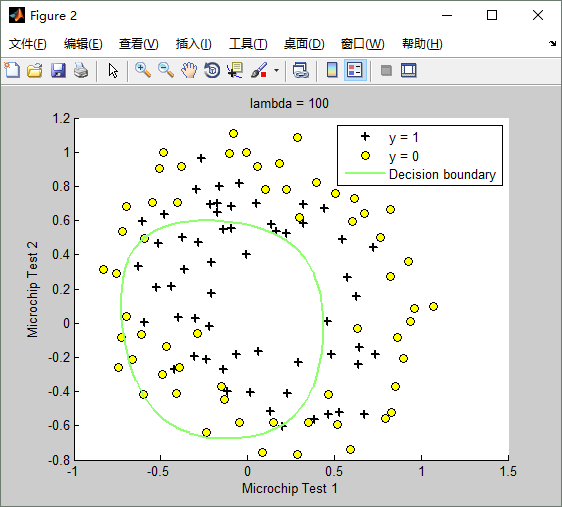
lambda(λ)==100时，训练出来的模型（hypothesis function）如下：Train Accuracy: 61.016949

---

1. Visualizing the data
   这部分使用的代码和上面的相同
   
   但这次的数据不能用直线来拟合出边界。
2. Feature mapping

使用已有的特征的幂来当做新的特征，这里最高6次幂。代码如下

function out = mapFeature(X1, X2)
 % MAPFEATURE Feature mapping function to polynomial features
 %
 %   MAPFEATURE(X1, X2) maps the two input features
 %   to quadratic features used in the regularization exercise.
 %
 %   Returns a new feature array with more features, comprising of 
 %   X1, X2, X1.^2, X2.^2, X1*X2, X1*X2.^2, etc..
 %
 %   Inputs X1, X2 must be the same size
 %
degree = 6;
out = ones(size(X1(:,1)));
for i = 1:degree
    for j = 0:i
        out(:, end+1) = (X1.^(i-j)).*(X2.^j);
    end
end

end

？？？？？？？？？？看不懂

1. Cost function and gradient
   公式如下
   
   theta_0和之前的相同，其余的参数在最后加了
   代码如下

hx = sigmoid(X * theta);
    J = (-1/m) * sum(y .* log(hx) + (1-y) .* log(1 - hx)) + ...
        (lambda/(2*m)) * (sum(theta .* theta) - theta(1)^2);

要注意减掉theta(1)的平方，因为公式中不包含 (theta_0)，所以需要去掉。

？？？？？？？？？？看不懂

梯度下降的算法公式

计算代码

function [J, grad] = costFunctionReg(theta, X, y, lambda)
    m = length(y); % number of training examples
    grad = zeros(size(theta));

    hx = sigmoid(X * theta);
    J = (-1/m) * sum(y .* log(hx) + (1-y) .* log(1 - hx)) + ...
        (lambda/(2*m)) * (sum(theta .* theta) - theta(1)^2);

    grad(1) = (1/m) * sum((hx - y) .* X(:, 1));
    n = length(theta);
    for j = 2 : n
        grad(j) = (1/m) * sum((hx - y) .* X(:, j)) + (lambda / m) * theta(j);
    end
end

1. plotDecisionBoundary
   画出非线性边界的代码

else
    % Here is the grid range
    u = linspace(-1, 1.5, 50);
    v = linspace(-1, 1.5, 50);

    z = zeros(length(u), length(v));
    % Evaluate z = theta*x over the grid
    for i = 1:length(u)
        for j = 1:length(v)
            z(i,j) = mapFeature(u(i), v(j))*theta;
        end
    end
    z = z'; % important to transpose z before calling contour

    % Plot z = 0
    % Notice you need to specify the range [0, 0]
    contour(u, v, z, [0, 0], 'LineWidth', 2)
end

**

？？？？？？？？？？？？？看不懂

**
5. change regularization parameters

修改ex2_reg.m第90行可以修改lambda的大小，等于0对应不进行正则化。

作业的关键代码

plotData

pos = find(y==1);
neg = find(y==0);
plot(X(pos,1),X(pos,2),'k+','Linewidth',2,'MarkerSize',7);
plot(X(neg,1),X(neg,2),'ko','MarkerFaceColor','y','MarkerSize',7);

sigmoid

g=1./(1+exp(-z));

costFunction

z=X*theta;
h=sigmoid(z);
J=sum(-y.*log(h)-(1-y).*log(1-h))/m;

grad=(1/m)*(X.'*(h-y));

predict

h = sigmoid(X * theta); 
p = (h >= 0.5); 

costFunctionReg

h=sigmoid(X*theta);
J=sum(-y.*log(h)-(1-y).*log(1-h))/m + (lambda/(2*m))*sum(theta(2:end).^2);

grad(1)=(1/m)*(X(:,1).'*(h-y));
grad(2:end) =(1/m)*(X(:,2:end).'*(h-y))+lambda*theta(2:end)/m;