Python-OpenCV ·学习笔记

注：笔记 来自课程 Python+OpenCV计算机视觉
Tips①：只是记录从这个课程学到的东西，不是推广、没有安利
Tips②：本笔记主要目的是为了方便自己遗忘查阅，或过于冗长、或有所缺省、或杂乱无章，见谅

一、基本操作

1、读取图像

img = cv2.imread("XX.jpg")

img = cv2.imread("XX.jpg", cv2.IMREAD_XXX)

2、展示图像

cv2.imshow("window_name", img)
cv2.waitKey(0)

3、保存图像

cv2.imwrite("XXX.jpg", img)

4、关闭全部窗口

用完cv记得destroyAllWindows

cv2.destroyAllWindows()

二、基本处理

1、访问像素

在img读取了图像后，可用img[]的形式访问相关区域像素值

img_bgr[15, 15]		# [168 145 219]
img_bgr[15, 15, 2]	# 219

img_gray[15, 15]	# 144

img_bgr[15, 15] = [255, 255, 255]
img_bgr[15:45, 15:45] = [255, 255, 255]

此外，也可以通过img.item()获取、通过img.itemset修改像素值

print(f"B：{img_bgr.item(15, 15, 0)}")
print(f"G：{img_bgr.item(15, 15, 1)}")
print(f"R：{img_bgr.item(15, 15, 2)}")

img_bgr.itemset((88, 99, 0), 155)

2、图像属性

形状

img.shape	# [400, 400, 3]

像素数

img.size	# 480000

图像类型

img.dtype	# uint8

3、图像ROI

ROI即感兴趣区域，从被处理的图像以方框、圆、椭圆、不规则多边形等方式勾勒出需要处理的区域。

可以通过切片访问img从而得到ROI区域

示例代码：

import cv2

'''读取图像'''
img1 = cv2.imread("../001.jpg")
img2 = cv2.imread("../002.jpg")

cv2.imshow("img1", img1)
cv2.imshow("img2", img2)

'''ROI区域获取'''
face = img1[50:230, 50:230]

'''观察ROI区域'''
cv2.imshow("face", face)

'''放入另一张图像'''
img2[40:220, 380:200:-1] = face
cv2.imshow("new_img2", img2)

'''关闭窗口'''
cv2.waitKey(0)
cv2.destroyAllWindows()

效果：

4、通道的拆分与合并

拆分通道

b, g, r = cv2.split(img)

合并通道

m = cv2.merge([b, g, r])

三、图像运算

1、图像加法

图像加法分为两种$\{\begin{array}{ll}取模加法& pt=(pt1+pt2)\%255\\ & \\ 饱和加法& pt=\{\begin{array}{ll}pt1+pt2& pt1+pt2\le 255\\ 255& pt1+pt2>255\end{array}\end{array}$

取模加法

img1 + img2

饱和加法

cv2.add(img1, img2)

示例代码：

import cv2

'''读取图像'''
img_a = cv2.imread("../001.jpg")
img_b = img_a
cv2.imshow("origin", img_a)

'''取模加法'''
res1 = img_a + img_b
cv2.imshow("res1", res1)

'''饱和加法'''
res2 = cv2.add(img_a, img_b)
cv2.imshow("res2", res2)

'''关闭窗口'''
cv2.waitKey(0)
cv2.destroyAllWindows()

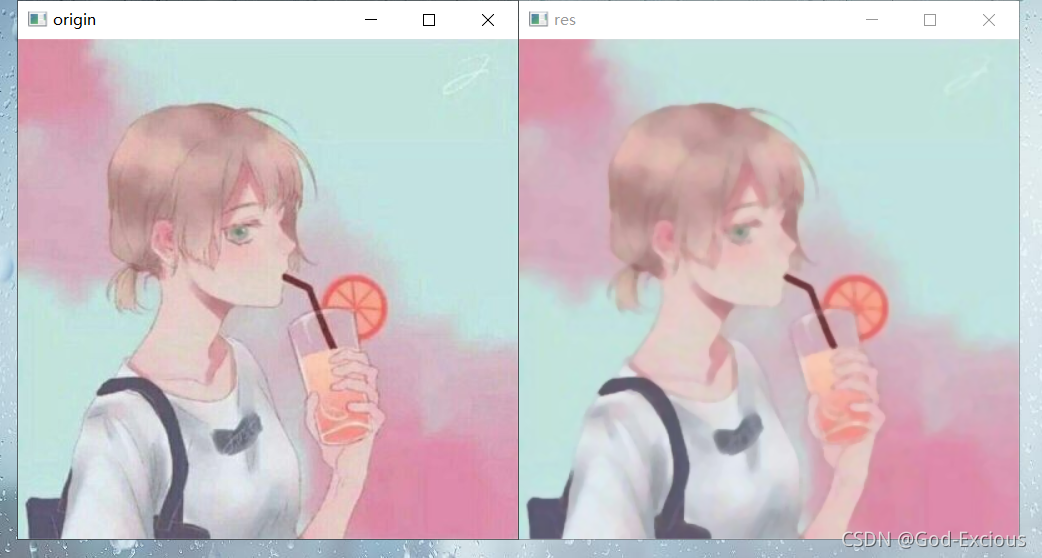
效果：

2、图像融合

图像融合公式：$\text{res}=\text{img1}\cdot \alpha +\text{img2}\cdot \beta +\gamma$

res = cv2.addWeighted(img1, alpha, img2, beta, gamma)

四、类型转换

OpenCV提供了200多种不同类型之间的转换。

'''BGR→Gray'''
img_gray = cv2.cvtColor(img, cv2.COLOR_BGR2GRAY)

'''Gray→BGR'''
img_bgr = cv2.cvtColor(img_gray, cv2.COLOR_GRAY2BGR)

'''BGR→RGB'''
img_rgb = cv2.cvtColor(img, cv2.COLOR_BGR2RGB)

五、几何变换

1、图像缩放

img_re = cv2.resize(img, (wid, hig))

img_re = cv2.resize(img, None, fx=0.5, fy=0.8)

2、图像翻转

img_res = cv2.flip(img, code)

示例代码：

import cv2

'''读取、展示图像'''
img = cv2.imread("../001.jpg")
cv2.imshow("origin", img)

'''图像缩放'''
img1 = cv2.flip(img, 0)     # 上下翻转（关于x轴）【flag = 0】
img2 = cv2.flip(img, 1)     # 左右翻转（关于y轴）【flag > 0】
img3 = cv2.flip(img, -1)    # 上下左右（关于原点）【flag < 0】
cv2.imshow("img1", img1)
cv2.imshow("img2", img2)
cv2.imshow("img3", img3)

'''等待、关闭窗口'''
cv2.waitKey(0)
cv2.destroyAllWindows()

效果：

3、图像平移

仿射变换

res = cv2.warpAffine(img, M, (wid, hig))

仿射原理
$$\text{res}[x,y]=\text{img}[M_{11}x+M_{12}y+M_{13},M_{21}x+M_{22}y+M_{23}]$$

图像平移

利用仿射变换，图像平移只需要设置平移矩阵$$M=\left[\begin{array}{ccc}1& 0& x\\ 0& 1& y\end{array}\right]$$其中，$x$、$y$ 分别为 $x$方向 和 $y$方向 需要平移的像素单位

M = np.float32([1, 0, x], [0, 1, y])
res = cv2.warpAffine(img, M, (wid, hig))

示例代码

import cv2
import numpy as np

'''读取、展示图像'''
img = cv2.imread("../001.jpg")
cv2.imshow("origin", img)

'''平移'''
M = np.float32([[1, 0, 100], [0, 1, 100]])
img1 = cv2.warpAffine(img, M, img.shape[:2])
cv2.imshow("img1", img1)

'''等待、关闭窗口'''
cv2.waitKey(0)
cv2.destroyAllWindows()

效果

4、图像旋转

与图像平移类似，同样需要借助于仿射变换实现

要完成图像旋转，只需要设置旋转矩阵$$\begin{array}{rl}& M=\left[\begin{array}{ccc}\alpha & \beta & (1-\alpha )\cdot \text{center}.x-\beta \cdot \text{center}.y\\ -\beta & \alpha & \beta \cdot \text{center}.x+(1-\alpha )\cdot \text{center}.y\end{array}\right]\\ & \\ & 其中，\{\begin{array}{l}\alpha =scale\cdot \cos angle\\ \beta =scale\cdot \sin angle\end{array}\end{array}$$

这样的矩阵可以通过cv的API直接计算获取

retval = cv2.getRotationMatrix2D(center, angle, scale)

示例代码

import cv2

'''读取、展示图像'''
img = cv2.imread("../001.jpg")
cv2.imshow("origin", img)

'''图像旋转'''
rows, cols, chn = img.shape
M = cv2.getRotationMatrix2D((rows // 2, cols // 2), 45, 0.5)
img1 = cv2.warpAffine(img, M, (rows, cols))
cv2.imshow("img1", img1)

'''等待、关闭窗口'''
cv2.waitKey(0)
cv2.destroyAllWindows()

效果

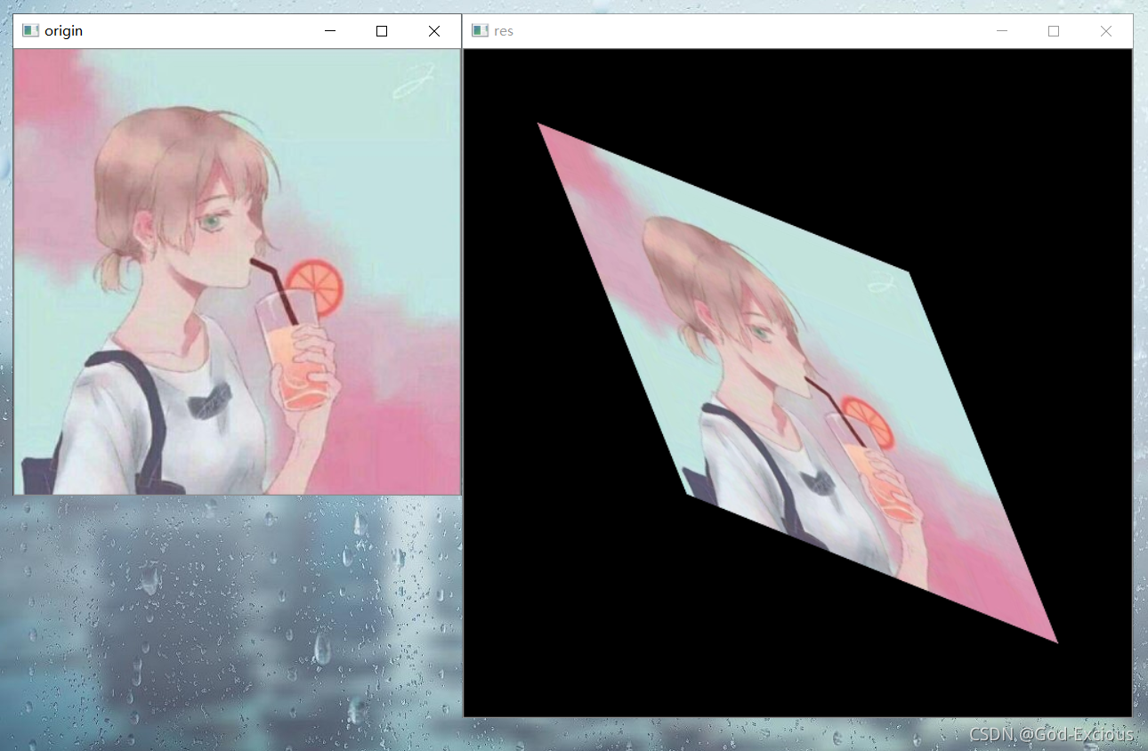
5、仿射变换

res = cv2.warpAffine(img, M, (wid, hig))

要确定一个仿射变换，主要是要确定一个变换矩阵$M$，而这里的矩阵$M$是一个$3\times 2$的矩阵，根据仿射原理$$\text{res}[x,y]=\text{img}[M_{11}x+M_{12}y+M_{13},M_{21}x+M_{22}y+M_{23}]$$
显然只需要三对点之间的映射关系就可以得到6个方程，从而确定矩阵$M$，以确定仿射变换

这样的矩阵可以通过cv的API直接计算获取

p1 = np.float32([[x1, y1], [x2, y2], [x3, y3]])
p2 = np.float32([[a1, b1], [a2, b2], [a3, b3]])
M = cv.getAffineTransform(p1, p2)

示例代码

import cv2
import numpy as np

'''读取、展示图像'''
img = cv2.imread("../001.jpg")
cv2.imshow("origin", img)

'''仿射变换'''
rows, cols = img.shape[:2]
p1 = np.float32([[0, 0], [rows - 1, 0], [0, cols - 1]])
p2 = np.float32([[rows // 6, cols // 6], [rows - 1, cols // 2], [rows // 2, cols - 1]])
M = cv2.getAffineTransform(p1, p2)
res = cv2.warpAffine(img, M, (round(rows * 1.5), round(cols * 1.5)))
cv2.imshow("res", res)

'''等待、关闭窗口'''
cv2.waitKey(0)
cv2.destroyAllWindows()

效果

六、阈值分割

1、阈值分割（基本概念）

• 二进制阈值化

  超过阈值设置为最大，小于阈值设置为 $0$

  $$dst(x,y)=\{\begin{array}{ll}\text{maxVal}& src(x,y)>\text{thresh}\\ 0& src(x,y)\le \text{thresh}\end{array}$$

  

• 反二进制阈值化

  超过阈值设置为 $0$，小于阈值设置为最大

  $$dst(x,y)=\{\begin{array}{ll}0& src(x,y)>\text{thresh}\\ \text{maxVal}& src(x,y)\le \text{thresh}\end{array}$$

  

• 截断阈值化

  大于等于阈值设置为阈值，小于阈值保持不变

  $$dst(x,y)=\{\begin{array}{ll}\text{threshold}& src(x,y)\ge \text{thresh}\\ src(x,y)& src(x,y)<\text{thresh}\end{array}$$

  

• 反阈值化为0

  大于等于阈值设置为 $0$，小于阈值保持不变

  $$dst(x,y)=\{\begin{array}{ll}0& src(x,y)\ge \text{thresh}\\ src(x,y)& src(x,y)<\text{thresh}\end{array}$$

  

• 阈值化为0

  大于等于阈值保持不变，小于阈值设置为 $0$

  $$dst(x,y)=\{\begin{array}{ll}src(x,y)& src(x,y)\ge \text{thresh}\\ 0& src(x,y)<\text{thresh}\end{array}$$

  

2、阈值分割（代码实现）

阈值分割

retval, dst = cv2.threshold(src, thresh, maxval, type)

示例代码

import cv2

'''读取图像'''
img = cv2.imread("001.jpg", cv2.IMREAD_GRAYSCALE)
cv2.imshow("origin", img)

'''阈值设置'''
thresh = 175

'''二进制阈值化'''
_, img_thresh_binary = cv2.threshold(img, thresh, 255, cv2.THRESH_BINARY)
cv2.imshow("thresh_binary", img_thresh_binary)

'''反二进制阈值化'''
_, img_thresh_binary_inv = cv2.threshold(img, thresh, 255, cv2.THRESH_BINARY_INV)
cv2.imshow("thresh_binary_inv", img_thresh_binary_inv)

'''截断阈值化'''
_, img_thresh_trunc = cv2.threshold(img, thresh, 255, cv2.THRESH_TRUNC)
cv2.imshow("thresh_trunc", img_thresh_trunc)

'''反阈值化为0'''
_, img_thresh_tozero_inv = cv2.threshold(img, thresh, 255, cv2.THRESH_TOZERO_INV)
cv2.imshow("thresh_tozero_inv", img_thresh_tozero_inv)

'''阈值化为0'''
_, img_thresh_tozero = cv2.threshold(img, thresh, 255, cv2.THRESH_TOZERO)
cv2.imshow("thresh_tozero", img_thresh_tozero)

'''等待、关闭图像'''
cv2.waitKey(0)
cv2.destroyAllWindows()

测试

七、图像平滑处理

作用：可以将图像模糊一些，以去除一些原来图像上明显的噪点

1、均值滤波

这个概念有点类似卷积神经网络里的卷积核

将某个像素周围的像素矩阵和核矩阵展平计算内积，得到一个新的像素值

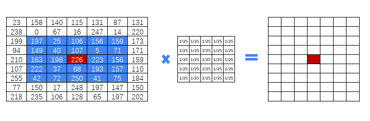
将整张图像进行这样的操作得到均值滤波后的图像

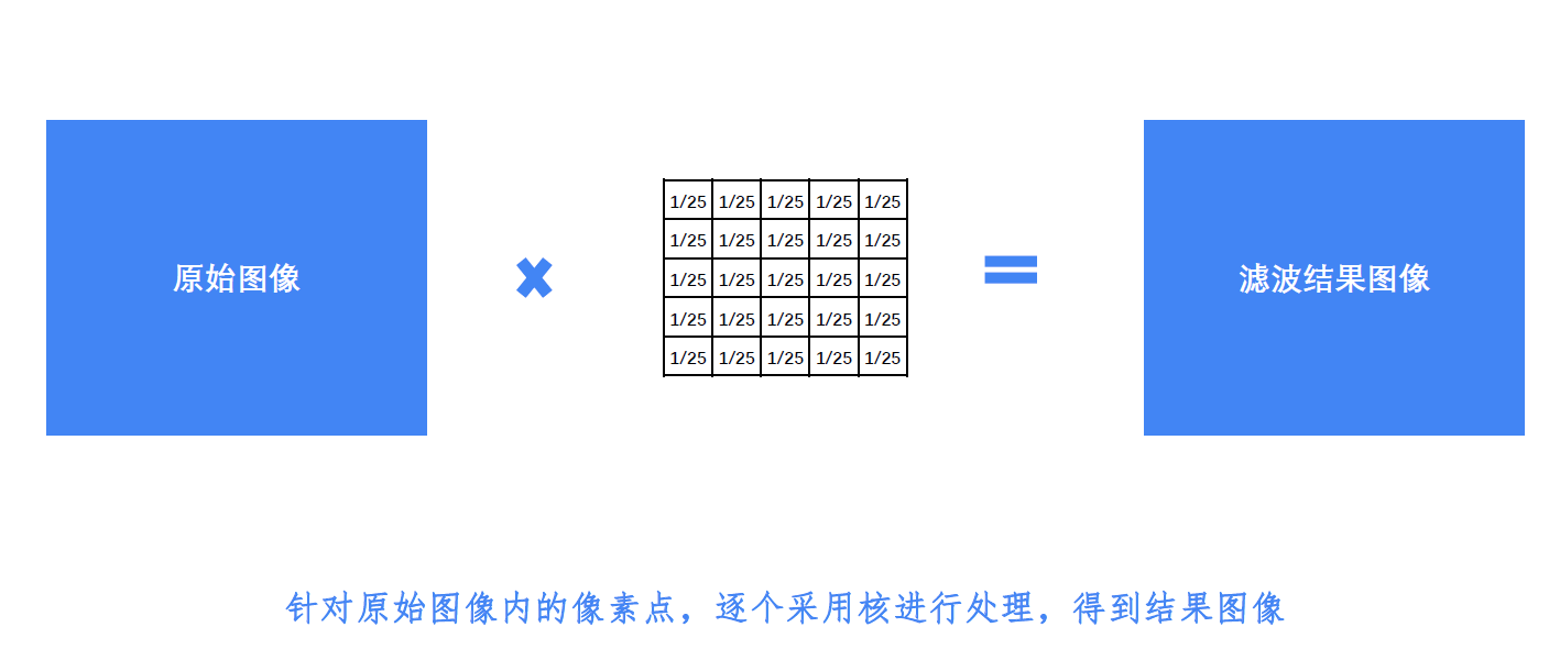
均值滤波

均值滤波实际上就是将周围的像素值计算平均值

res = cv2.blur(img, (Ksize, Ksize))

示例代码

import cv2

'''读取图像'''
img = cv2.imread("../001.jpg")
cv2.imshow("origin", img)

'''均值滤波'''
res = cv2.blur(img, (5, 5))
cv2.imshow("res", res)

'''等待、关闭图像'''
cv2.waitKey(0)
cv2.destroyAllWindows()

效果

2、方框滤波

方框滤波

res = cv2.boxFilter(img, -1, (Ksize, Ksize), normalize=True)		# 求和后求均值（等同均值滤波）
res = cv2.boxFilter(img, -1, (Ksize, Ksize), normalize=False)		# 求和（容易溢出）

示例代码

import cv2

'''读取图像'''
img = cv2.imread("../001.jpg")

'''先预处理一下'''
img = cv2.multiply(img, (1, 1, 1, 1), scale=0.36)
cv2.imshow("origin", img)

'''方框滤波'''
res = cv2.boxFilter(img, -1, (2, 2), normalize=False)
cv2.imshow("res", res)

'''等待、关闭图像'''
cv2.waitKey(0)
cv2.destroyAllWindows()

效果

3、高斯滤波

高斯滤波

相当于在均值滤波的基础上增加了权重的概念，可以看做是加权均值滤波

'''
Ksize		必须为奇数
sigmaX		X方向方差，控制权重
			sigmaX = 0时， sigma = 0.3 * ((Ksize - 1) * 0.5 - 1) + 0.8
'''
res = cv2.GaussianBlur(img, (Ksize, Ksize), sigmaX)

示例代码

import cv2

'''读取图像'''
img = cv2.imread("../001.jpg")
cv2.imshow("origin", img)

'''高斯滤波'''
res = cv2.GaussianBlur(img, (5, 5), 0)
cv2.imshow("res", res)

'''等待、关闭图像'''
cv2.waitKey(0)
cv2.destroyAllWindows()

效果

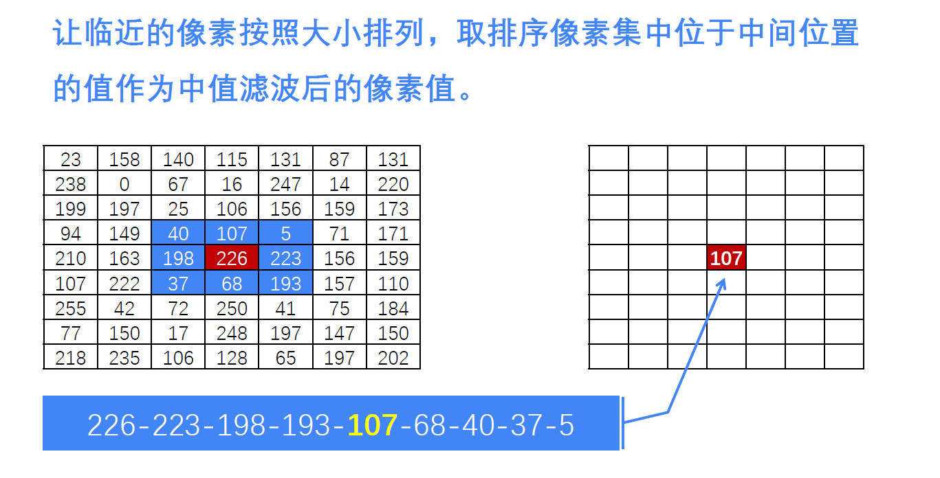
4、中值滤波

中值滤波

将像素附近、核大小内的元素排序后的中间值作为处理后的相应的像素

'''
Ksize必须为奇数
'''
res = cv2.medianBlur(img, Ksize)

示例代码

import cv2

'''读取图像'''
img = cv2.imread("../001.jpg")
cv2.imshow("origin", img)

'''中值滤波'''
res = cv2.medianBlur(img, 5)
cv2.imshow("res", res)

'''等待、关闭图像'''
cv2.waitKey(0)
cv2.destroyAllWindows()

效果

5、卷积

卷积

可以看做自定义核的矩阵，进行相关运算

res = cv2.filter2D(img, -1, Kernel)

示例代码

import cv2
import numpy as np

'''读取图像'''
img = cv2.imread("../001.jpg")
cv2.imshow("origin", img)

'''卷积'''
kernel = np.array([[0.05, 0.05, 0.3], [0.3, 0.02, 0.01], [0, 0, 0]]) * 2
res = cv2.filter2D(img, -1, kernel)
cv2.imshow("res", res)

'''等待、关闭图像'''
cv2.waitKey(0)
cv2.destroyAllWindows()

效果

八、形态学处理

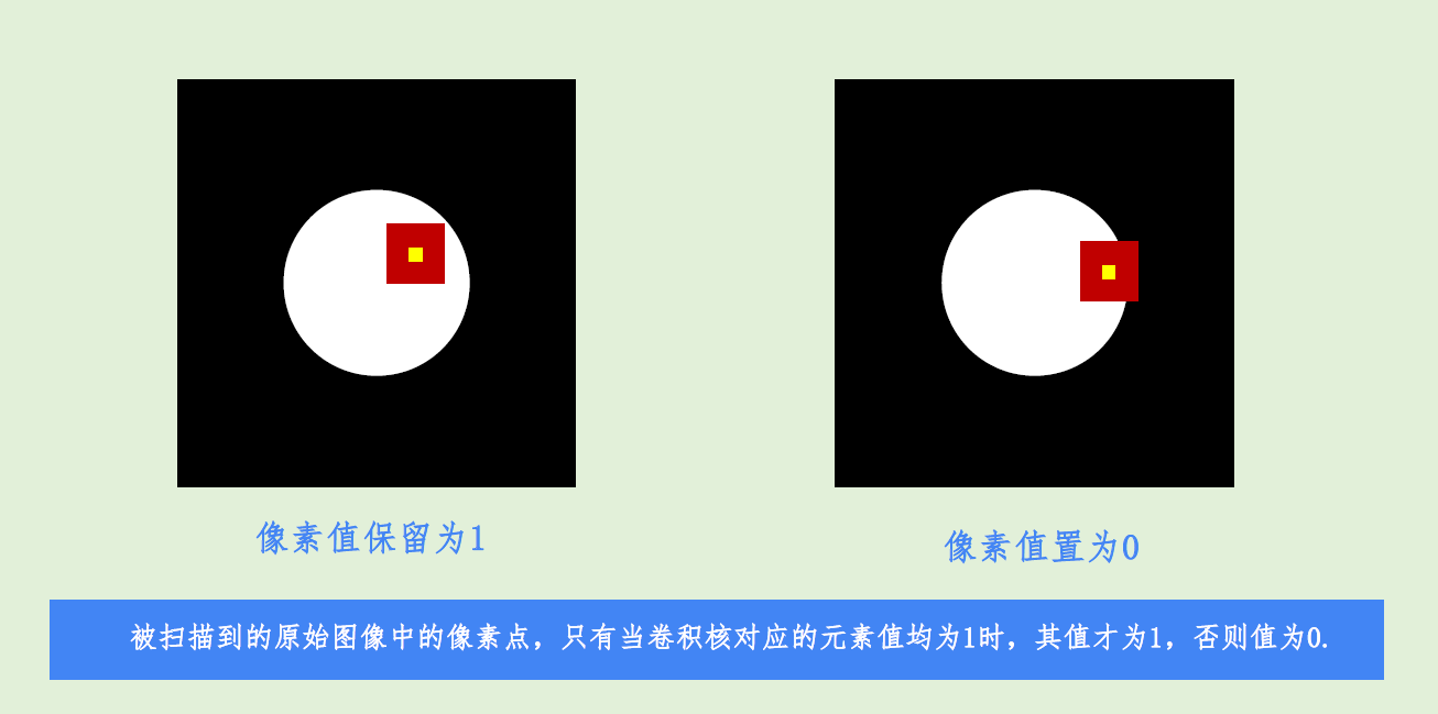
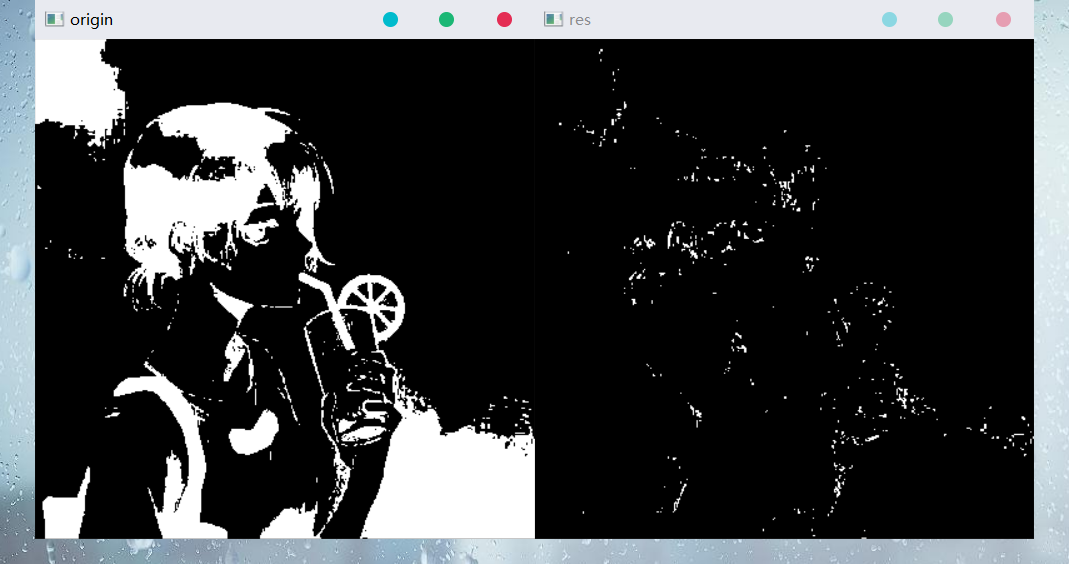
1、图像腐蚀

腐蚀

该操作一般针对二值图像

腐蚀操作需要两个输入对象：二值图像、卷积核

基本操作：卷积核遍历图像的一部分，当卷积核内的元素均为1时，结果图像对应位置的像素值才为1，否则为0（腐蚀掉白色的边缘）

如下图所示：

'''
iterations	迭代次数
'''
res = cv2.erode(img, kernel, iterations)

示例代码：

import cv2
import numpy as np

'''读取图像'''
img = cv2.imread("../001.jpg", cv2.IMREAD_GRAYSCALE)
_, img = cv2.threshold(img, 180, 255, cv2.THRESH_BINARY_INV)
cv2.imshow("origin", img)

'''腐蚀'''
kernel = np.ones((3, 3), np.uint8)
res = cv2.erode(img, kernel, iterations=9)
cv2.imshow("res", res)

'''等待、关闭图像'''
cv2.waitKey(0)
cv2.destroyAllWindows()

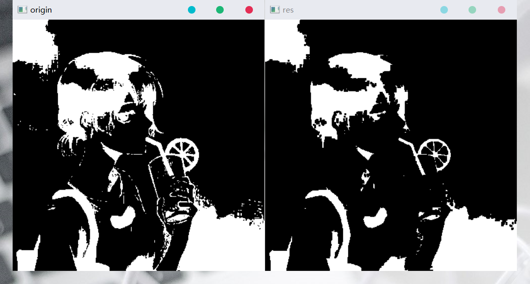
效果：

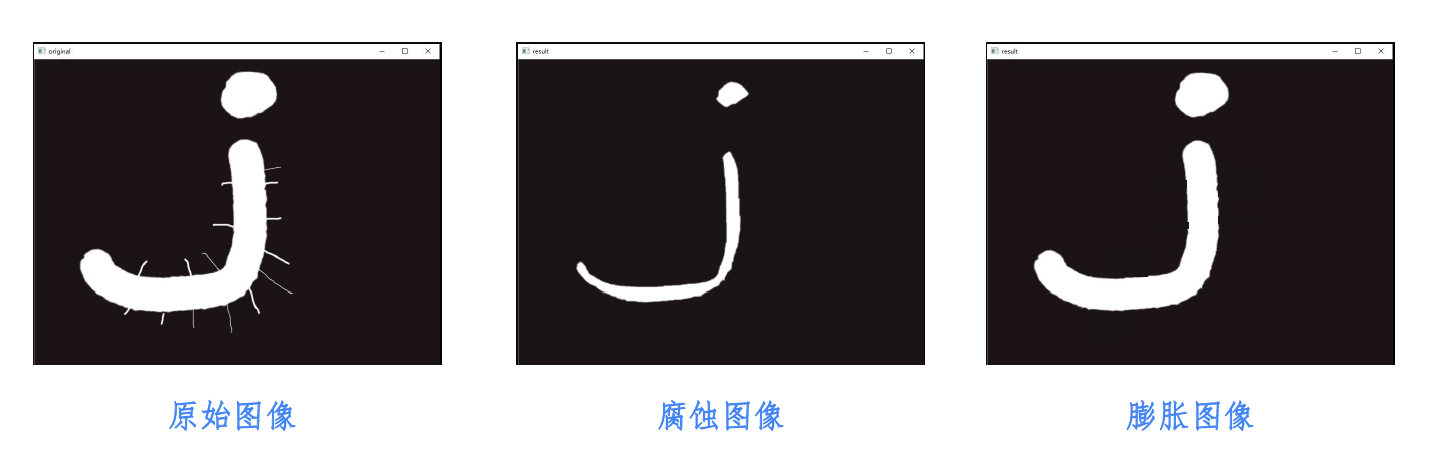
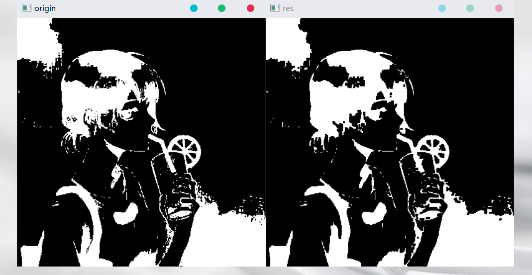
2、图像膨胀

膨胀

腐蚀操作的逆操作（同样针对二值图像，对白色的边缘进行膨胀）

作用：

• 图像被腐蚀后，去除了噪声，但是会压缩图像

• 对腐蚀后的图像，进行膨胀处理，可以去除噪声，并保持原有形状

  

res = cv2.dilate(img, kernel, iterations)

示例代码：

import cv2
import numpy as np

'''读取图像'''
img = cv2.imread("../001.jpg", cv2.IMREAD_GRAYSCALE)
_, img = cv2.threshold(img, 180, 255, cv2.THRESH_BINARY_INV)
cv2.imshow("origin", img)

'''膨胀'''
kernel = np.ones((3, 3), np.uint8)
res = cv2.dilate(img, kernel)
cv2.imshow("res", res)

'''等待、关闭图像'''
cv2.waitKey(0)
cv2.destroyAllWindows()

效果：

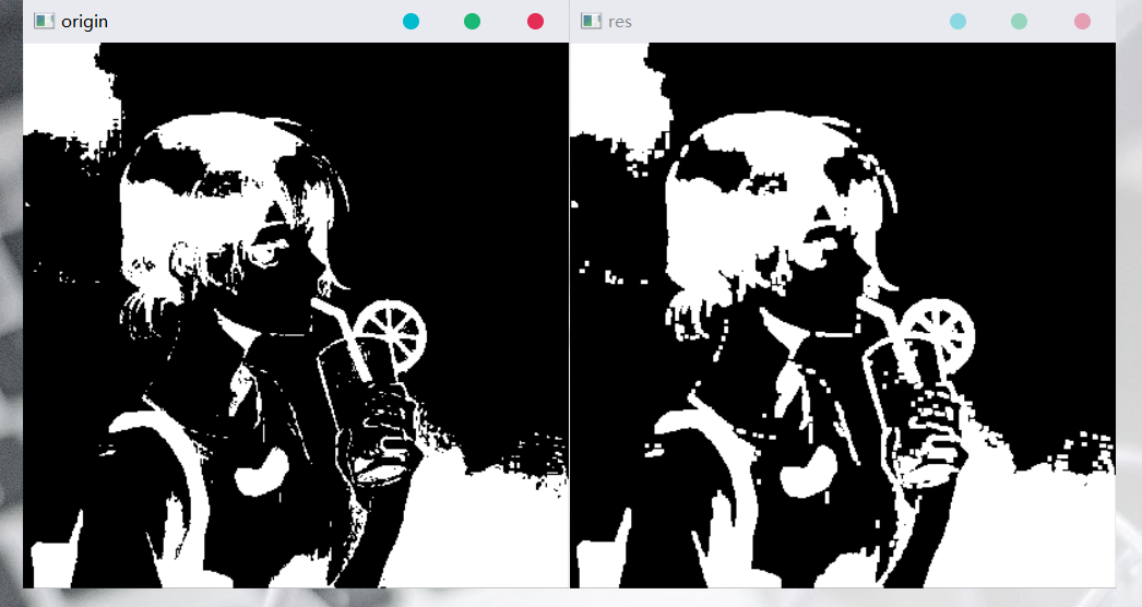
3、开运算

开运算

开运算的操作就相当于对图像先进行腐蚀再进行膨胀

开运算有助于去除图像的噪声

可以使用形态学扩展的API来实现开运算

res = cv2.morphologyEx(img, cv2.MORPH_OPEN, kernel)

示例代码：

import cv2
import numpy as np

'''读取图像'''
img = cv2.imread("../001.jpg", cv2.IMREAD_GRAYSCALE)
_, img = cv2.threshold(img, 180, 255, cv2.THRESH_BINARY_INV)
cv2.imshow("origin", img)

'''开运算'''
kernel = np.ones((3, 3), np.uint8)
res = cv2.morphologyEx(img, cv2.MORPH_OPEN, kernel)
cv2.imshow("res", res)

'''等待、关闭图像'''
cv2.waitKey(0)
cv2.destroyAllWindows()

效果：

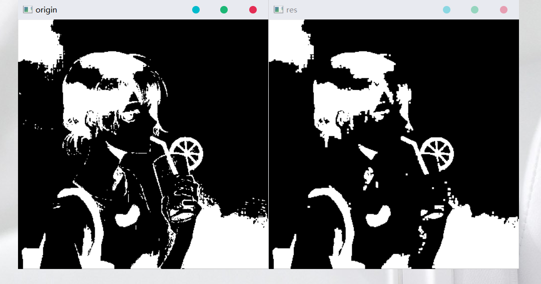
4、闭运算

闭运算的操作就相当于对图像先进行膨胀再进行腐蚀

闭运算有助于去除图像的内部的小孔、小黑点

可以使用形态学扩展的API来实现闭运算

res = cv2.morphologyEx(img, cv2.MORPH_CLOSE, kernel)

示例代码：

import cv2
import numpy as np

'''读取图像'''
img = cv2.imread("../001.jpg", cv2.IMREAD_GRAYSCALE)
_, img = cv2.threshold(img, 180, 255, cv2.THRESH_BINARY_INV)
cv2.imshow("origin", img)

'''闭运算'''
kernel = np.ones((3, 3), np.uint8)
res = cv2.morphologyEx(img, cv2.MORPH_CLOSE, kernel)
cv2.imshow("res", res)

'''等待、关闭图像'''
cv2.waitKey(0)
cv2.destroyAllWindows()

效果：

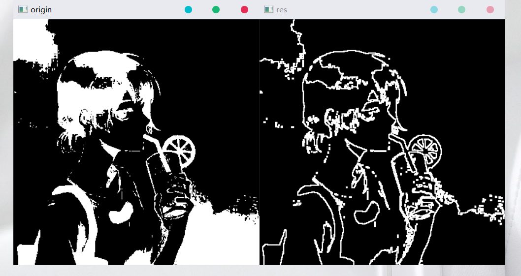
5、梯度运算

梯度运算

梯度运算的操作就相当于用膨胀图像减去腐蚀图像，可以得到图像的边缘信息

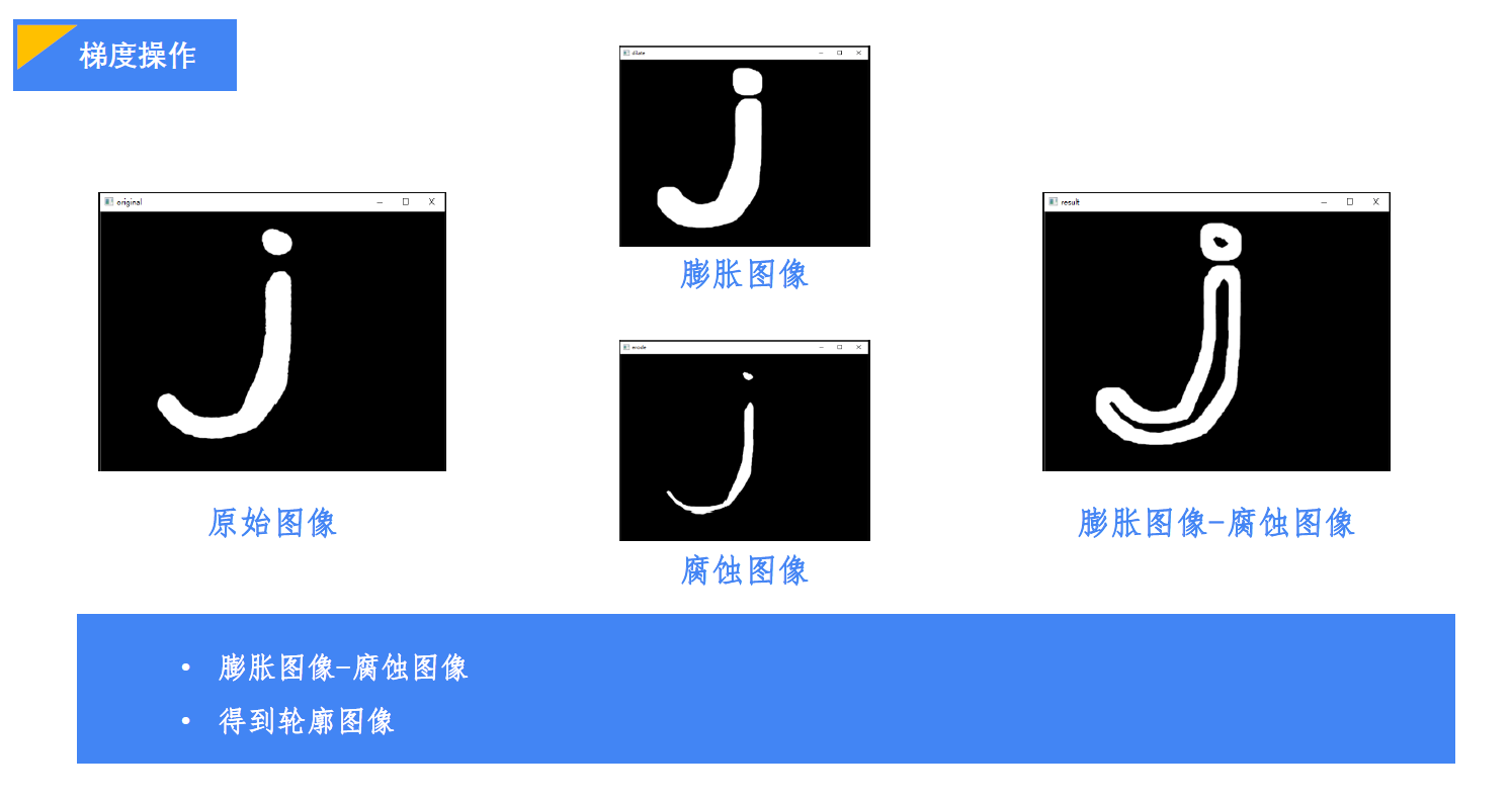
可以使用形态学扩展的API来实现梯度运算

res = cv2.morphologyEx(img, cv2.MORPH_GRADIENT, kernel)

示例代码：

import cv2
import numpy as np

'''读取图像'''
img = cv2.imread("../001.jpg", cv2.IMREAD_GRAYSCALE)
_, img = cv2.threshold(img, 180, 255, cv2.THRESH_BINARY_INV)
cv2.imshow("origin", img)

'''梯度运算'''
kernel = np.ones((3, 3), np.uint8)
res = cv2.morphologyEx(img, cv2.MORPH_GRADIENT, kernel)
cv2.imshow("res", res)

'''等待、关闭图像'''
cv2.waitKey(0)
cv2.destroyAllWindows()

效果：

6、礼帽运算（顶帽运算）

礼帽运算

礼帽运算的操作就相当于用原始图像减去开运算图像，可以得到图像的噪声信息（噪声图像）

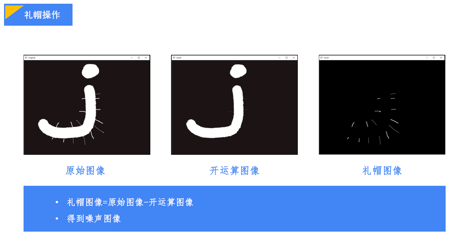
可以使用形态学扩展的API来实现礼帽运算

res = cv2.morphologyEx(img, cv2.MORPH_TOPHAT, kernel)

示例代码：

import cv2
import numpy as np

'''读取图像'''
img = cv2.imread("../001.jpg", cv2.IMREAD_GRAYSCALE)
_, img = cv2.threshold(img, 180, 255, cv2.THRESH_BINARY_INV)
cv2.imshow("origin", img)

'''礼帽运算'''
kernel = np.ones((3, 3), np.uint8)
res = cv2.morphologyEx(img, cv2.MORPH_TOPHAT, kernel)
cv2.imshow("res", res)

'''等待、关闭图像'''
cv2.waitKey(0)
cv2.destroyAllWindows()

效果：

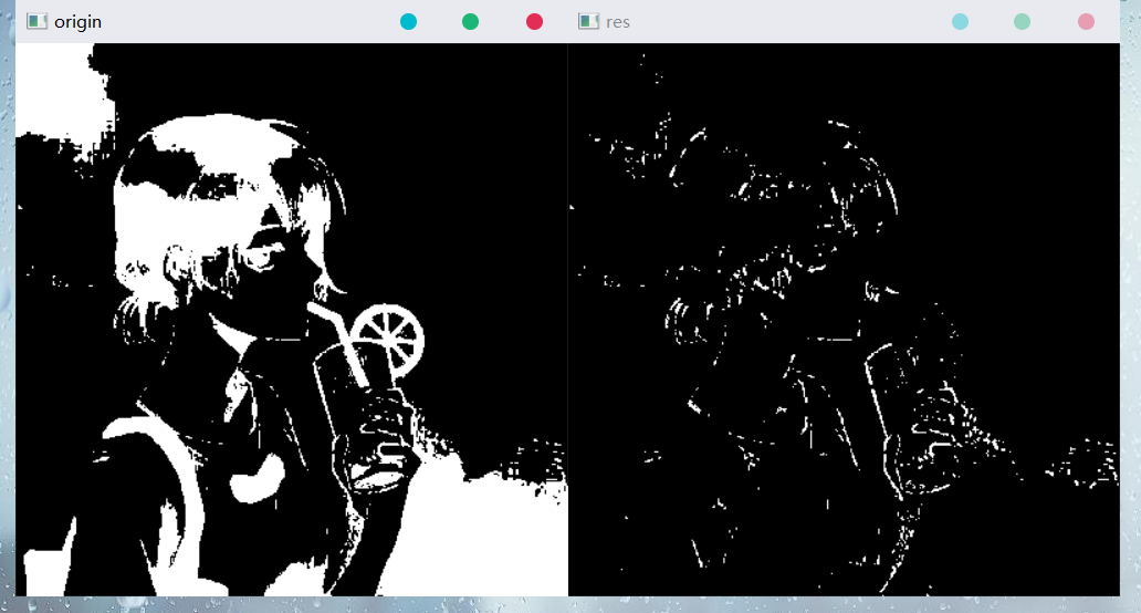
7、黑帽运算

黑帽运算

黑帽运算的操作就相当于用闭运算图像减去原始图像，可以得到图像内部的小孔、小黑点

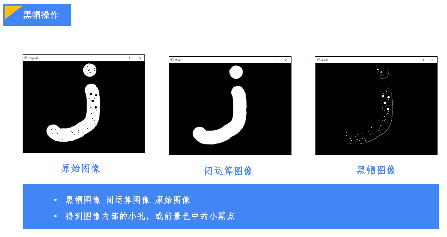
可以使用形态学扩展的API来实现礼帽运算

res = cv2.morphologyEx(img, cv2.MORPH_BLACKHAT, kernel)

示例代码：

import cv2
import numpy as np

'''读取图像'''
img = cv2.imread("../001.jpg", cv2.IMREAD_GRAYSCALE)
_, img = cv2.threshold(img, 180, 255, cv2.THRESH_BINARY_INV)
cv2.imshow("origin", img)

'''礼帽运算'''
kernel = np.ones((3, 3), np.uint8)
res = cv2.morphologyEx(img, cv2.MORPH_BLACKHAT, kernel)
cv2.imshow("res", res)

'''等待、关闭图像'''
cv2.waitKey(0)
cv2.destroyAllWindows()

效果：

九、图像梯度

1、sobel算子

理论基础

使用一个卷积核$G_x=\left[\begin{array}{ccc}-1& 0& 1\\ -2& 0& 2\\ -1& 0& 1\end{array}\right]$，使其与图像部分$\left[\begin{array}{ccc}{P}_1& P_2& P_3\\ P_4& P_5& P_6\\ P_7& P_8& P_9\end{array}\right]$转置后进行乘法，即可得到图像部分的中心点$P_5$处的$x$方向的梯度${P_5}_x$（这里的$G_x$在靠近中心$P_5$的$P_4$和$P_6$选择了更大的权重$2$）

这样的计算可以用于$x$方向上的边界检测：

• 如果${P_5}_x$很大，说明在$P_5$点右边的像素值和左边的像素值差别很大，就说明$P_5$是$x$方向上的一个边界点
• 如果${P_5}_x$很小，说明在$P_5$点右边的像素值和左边的像素值差别不大，就说明$P_5$不是$x$方向上的一个边界点

类似的，也还有$y$方向上的梯度，可以用一个卷积核$G_y$来进行计算

那么就可以根据$G_x$和$G_y$来计算一个图像的梯度，即$$G=\sqrt{{G_x}^2+{G_y}^2}$$

此外，也可以简化为$$G=|G_x|+|G_y|$$

这就是我们所谓的sobel算子

同样，对于某个具体的点的sobel算子也有$${P_5}_{\text{sobel}}=|{P_5}_x|+|{P_5}_y|$$

Tips：关于【为什么要加上绝对值、如何对图像深度进行设置、如何取绝对值】

• 如果直接计算，可能会出现负值，比如-255，那就很有可能被截断为0，而无法识别出其为边界点，因此，需要加上绝对值
  

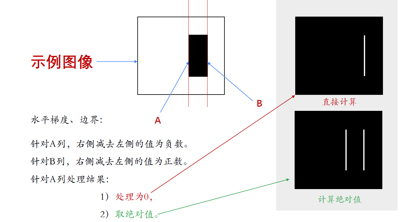
• 实际操作中，计算梯度值可能出现负数，通常处理的图像是np.uint8类型（cv2.CV_8U），如果结果也是该类型，所有负数会自动截断为0，从而发生信息丢失，所以，在计算时，深度参数ddepth可以使用更高的数据类型cv2.CV_64F来保留负数的值，取绝对值后，再转换为np.uint8类型（cv2.CV_8U）

• 将原始图像转换为256色位图（负值取绝对值）

  res = cv2.convertSacleAbs(img[, alpha[, beta]])
  
  '''一般只用把图像传入即可'''
  res = cv2.convertSacleAbs(img)
  

---

sobel算子

'''
ddepth	处理结果图像深度
		通常情况下，可以将该参数的值设置为-1，让处理结果与原始图像保持一致
dx,dy	表示要计算x轴方向、y轴方向的梯度
		要计算x轴方向梯度——dx=1, dy=0
		要计算x轴方向梯度——dx=0, dy=1
ksize	卷积核大小（一般不用，要用可以设置为奇数）
'''
res = cv2.Sobel(img, ddepth, dx, dy, [ksize])

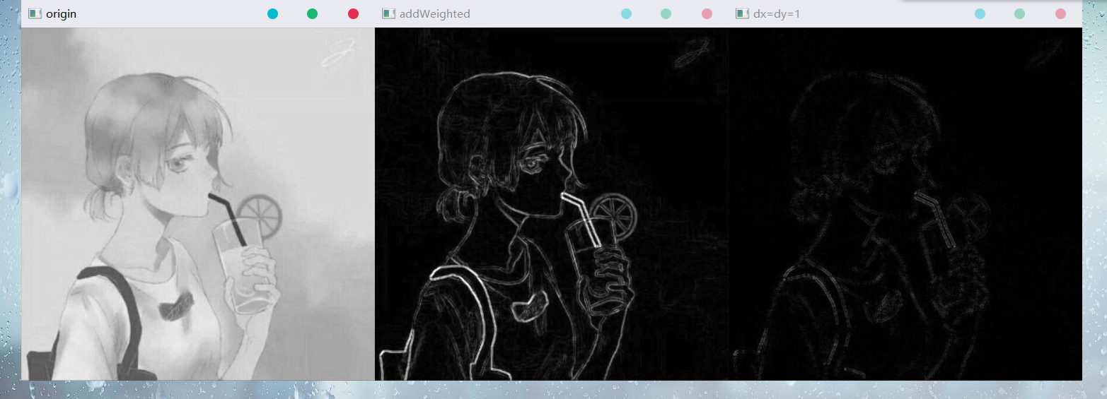
'''处理方式1（不能很好地处理边界）'''
res = cv2.Sobel(img, ddepth, 1, 1)

'''处理方式2（采用加权和的方式计算，可以很好地处理函数的边界问题）'''
dx = cv2.Sobel(img, ddepth, 1, 0)
dy = cv2.Sobel(img, ddepth, 0, 1)
# res = dx * 系数1 + dy * 系数2
res = cv2.addWeighted(dx, alpha, dy, beta, gamma)

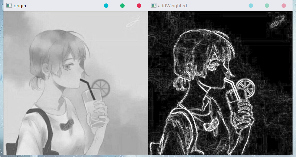
示例代码：

import cv2
import numpy as np

'''读取图像'''
img = cv2.imread("../001.jpg", cv2.IMREAD_GRAYSCALE)
cv2.imshow("origin", img)

'''sobel算子'''
dx = cv2.Sobel(img, cv2.CV_64F, 1, 0)
dy = cv2.Sobel(img, cv2.CV_64F, 0, 1)
dx = cv2.convertScaleAbs(dx)
dy = cv2.convertScaleAbs(dy)
res1 = cv2.addWeighted(dx, 0.5, dy, 0.5, 0)
cv2.imshow("addWeighted", res1)

sobel = cv2.Sobel(img, cv2.CV_64F, 1, 1)
res2 = cv2.convertScaleAbs(sobel)
cv2.imshow("dx=dy=1", res2)

'''等待、关闭图像'''
cv2.waitKey(0)
cv2.destroyAllWindows()

效果：

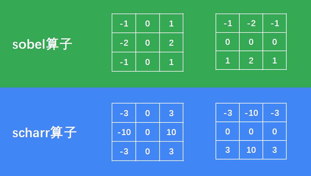
2、scharr算子

理论基础

在使用$3\times 3$的sobel算子时，可能不太精确，可以使用如下的scharr算子，效果更好：

$$\begin{array}{rl}& G_x=\left[\begin{array}{ccc}-3& 0& 3\\ -10& 0& 10\\ -3& 0& 3\end{array}\right]\\ & \\ & G_y=\left[\begin{array}{ccc}-3& -10& -3\\ 0& 0& 0\\ 3& 10& 3\end{array}\right]\end{array}$$

---

scharr算子

'''
dx,dy	dx表示x轴方向，dy表示y轴方向
		需要满足 dx>=0, dy>=0, dx+dy==1
		
scharr其实是改进的sobel算子
	res = cv2.Scharr(img, ddepth, dx, dy)
	实际上就等价于
	res = cv2.Sobel(img, ddepth, dx, dy, -1)
'''
res = cv2.Scharr(img, ddepth, dx, dy)

示例代码：

import cv2
import numpy as np

'''读取图像'''
img = cv2.imread("../001.jpg", cv2.IMREAD_GRAYSCALE)
cv2.imshow("origin", img)

'''scharr算子'''
dx = cv2.Scharr(img, cv2.CV_64F, 1, 0)
dy = cv2.Scharr(img, cv2.CV_64F, 0, 1)
dx = cv2.convertScaleAbs(dx)
dy = cv2.convertScaleAbs(dy)
res1 = cv2.addWeighted(dx, 0.5, dy, 0.5, 0)
cv2.imshow("addWeighted", res1)

'''等待、关闭图像'''
cv2.waitKey(0)
cv2.destroyAllWindows()

效果：

3、laplacian算子（拉普拉斯算子）

理论基础

拉普拉斯算子类似于二阶sobel导数（2次右边减左边、2次下边减上边）

其使用的卷积核为

$$G=\left[\begin{array}{ccc}0& 1& 0\\ 1& -4& 1\\ 0& 1& 0\end{array}\right]$$

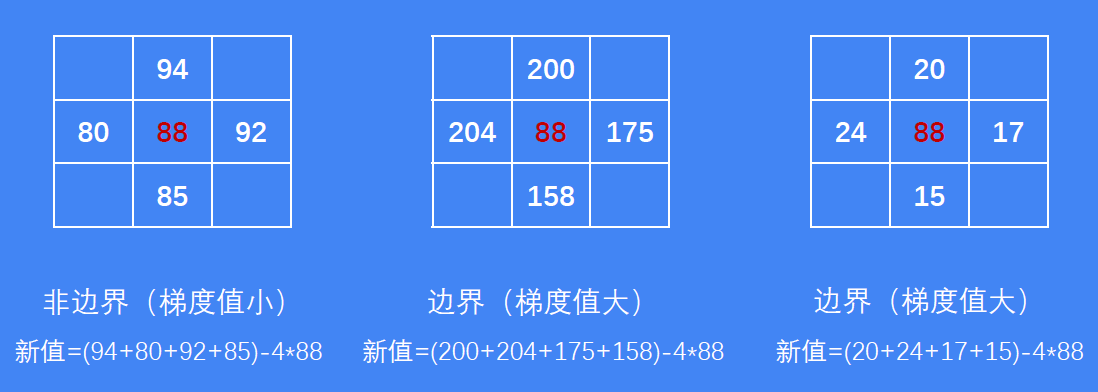
其所计算的某一点的梯度示意如下

$$\begin{array}{rl}& \left[\begin{array}{ccc}{P}_1& P_2& P_3\\ P_4& P_5& P_6\\ P_7& P_8& P_9\end{array}\right]\\ & \\ & {P_5}_{new}=(P_2+P_4+P_6+P_8)-4\ast P_5\end{array}$$

同样，laplacian算子可以用于检测边界

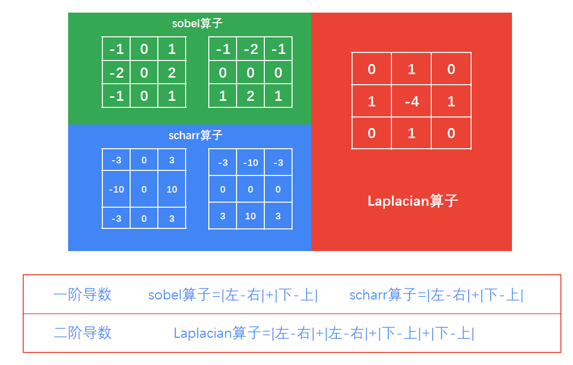
sobel算子、scharr算子、laplacian算子的比较：

---

laplacian算子

res = cv2.Laplacian(img, ddepth)

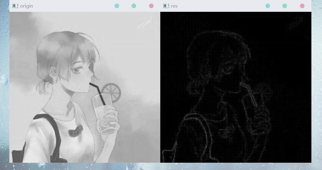
示例代码：

import cv2
import numpy as np

'''读取图像'''
img = cv2.imread("../001.jpg", cv2.IMREAD_GRAYSCALE)
cv2.imshow("origin", img)

'''laplacian算子'''
res = cv2.Laplacian(img, cv2.CV_64F)
res = cv2.convertScaleAbs(res)
cv2.imshow("res", res)

'''等待、关闭图像'''
cv2.waitKey(0)
cv2.destroyAllWindows()

效果：

十、Canny边缘检测

Canny边缘检测的一般步骤

1. 去噪：
   边缘检测容易受到噪声的影响，因此，在边缘检测之前，需要先进行去噪
   通常使用高斯滤波进行去噪

2. 梯度：
   

   示例：
   

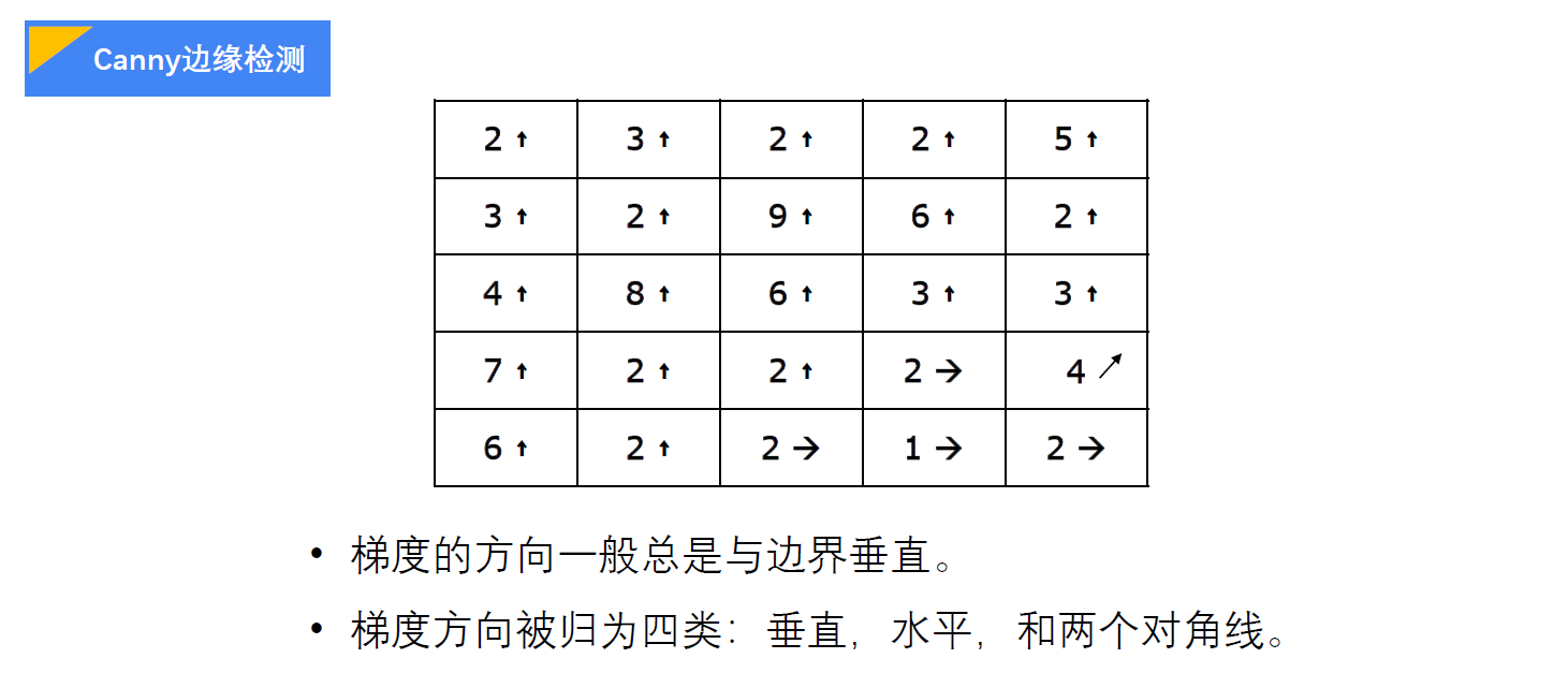
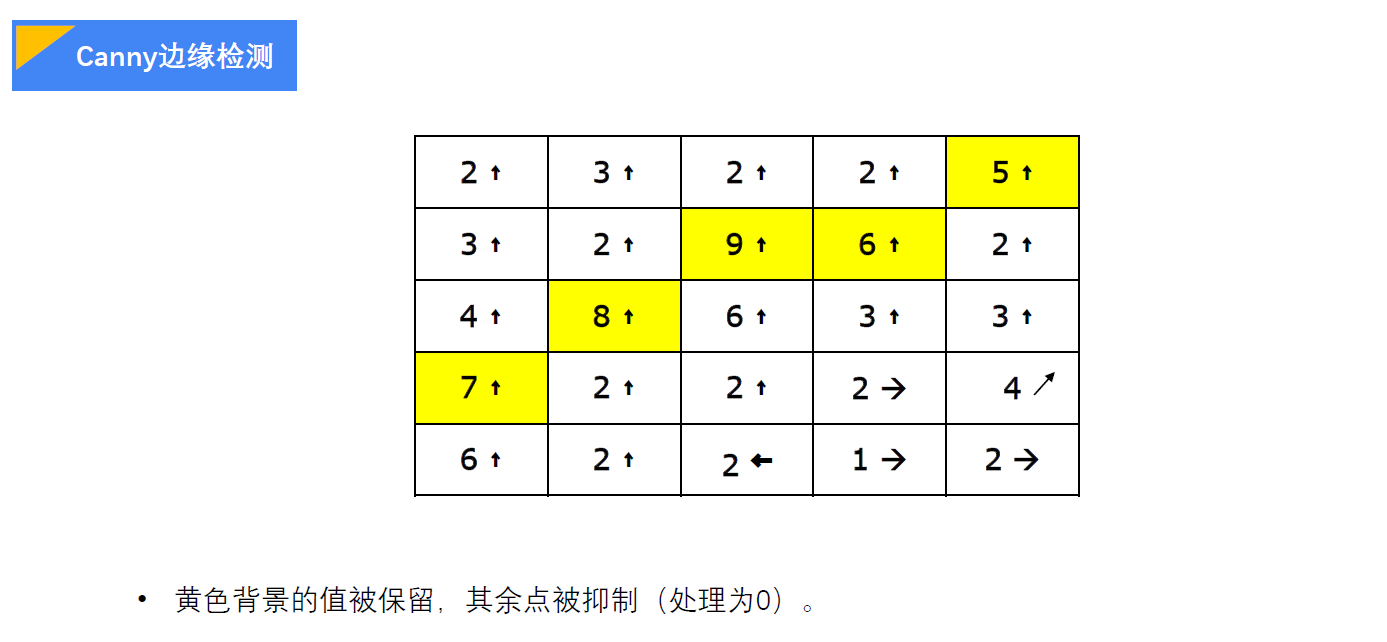
3. 非极大值抑制：
   在获得了梯度和方向后，遍历图像，去除所有非边界点

   实现方式：逐个遍历像素点，判断当前像素点是否是周围像素点中具有相同方向梯度的最大值（最大——保留，非最大——抛弃）

   示例：
   

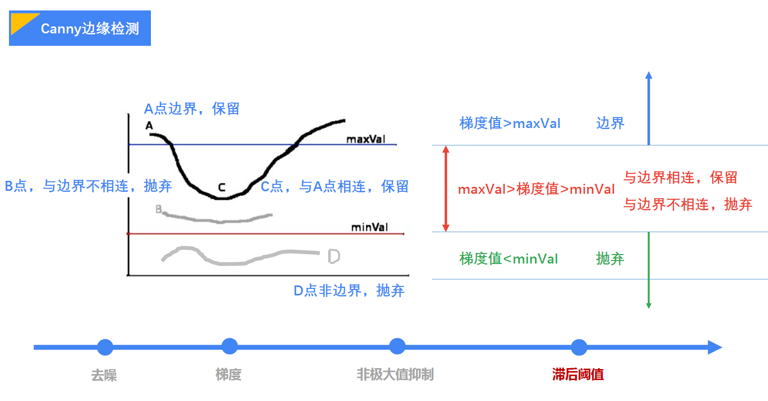
4. 滞后阈值：
   需要设置两个滞后阈值：minval、maxval
   根据剩余的点的梯度值与其相连情况判断，决定是保留/抛弃这个点
   

---

Canny边缘检测

'''
Tips：
	如果想让Canny边缘检测的边更多（细节更丰富），可以把这两个值调低
	如果想让Canny边缘检测的边少一些（细节不丰富），可以把这两个值调高
'''
res = cv2.Canny(img, threshold1, threshold2)

示例代码：

import cv2
import numpy as np

'''读取图像'''
img = cv2.imread("001.jpg", cv2.IMREAD_GRAYSCALE)
cv2.imshow("origin", img)

'''Canny边缘检测'''
res = cv2.Canny(img, 100, 200)
cv2.imshow("res", res)

'''等待、关闭图像'''
cv2.waitKey(0)
cv2.destroyAllWindows()

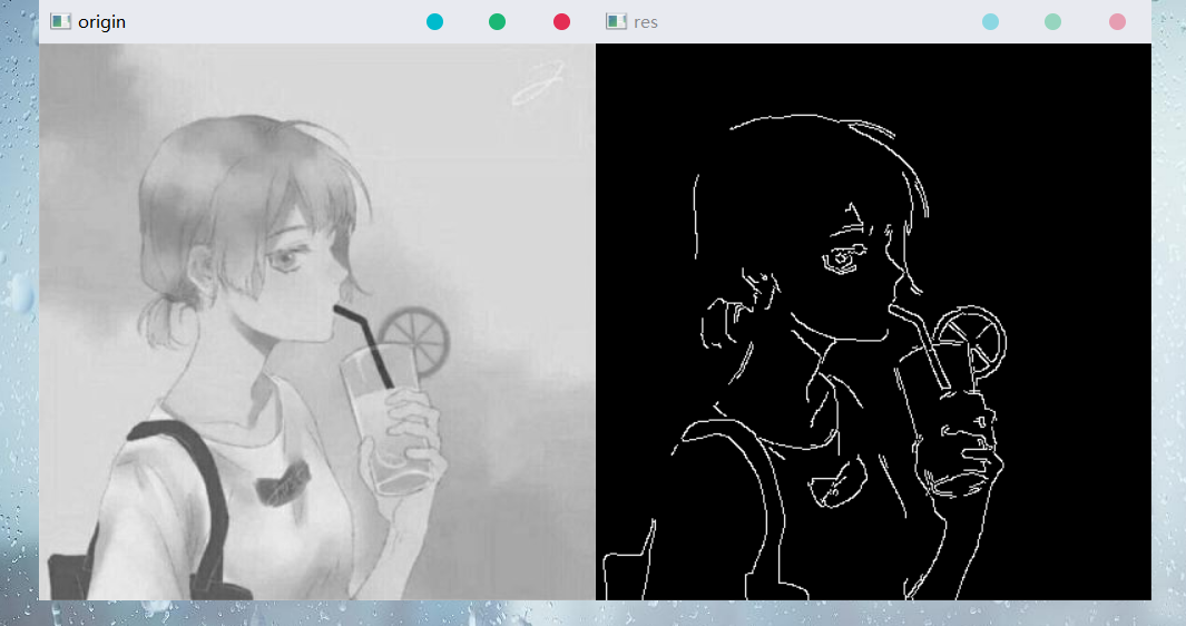
效果：

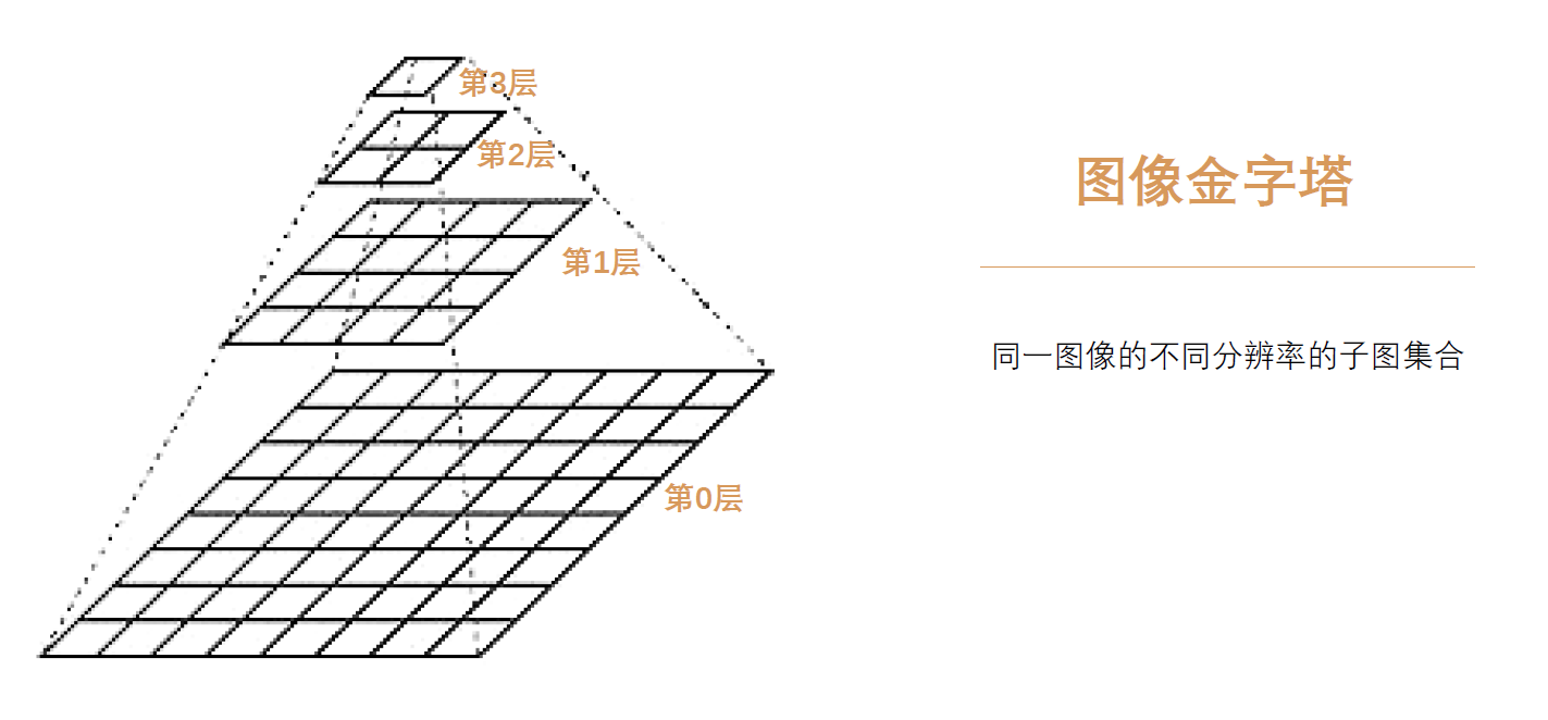
十一、图像金字塔

图像金字塔

• 图像金字塔指的是由同一图像的不同分辨率的子图构成的集合
  

• 生成图像金字塔的方法有两种——下采样（缩小）、上采样（放大）

1、高斯金字塔

下采样

• 下采样即从第$i$层（$G_i$）获取第$i+1$层（$G_{i+1}$）

• 下采样的一般步骤如下：
  ①、对图像$G_i$进行高斯核卷积
  $$\text{kernel}=\frac{1}{256}\left[\begin{array}{ccccc}1& 4& 6& 4& 1\\ 4& 16& 24& 16& 4\\ 6& 24& 36& 24& 6\\ 4& 16& 24& 16& 4\\ 1& 4& 6& 4& 1\end{array}\right]$$
  显然，距离中心点越近，权重越大

  ②、删除所有偶数行和列

• 每次处理后，原始图像会从$\text{M}\times \text{N}$变为$\frac{\text{M}}{2}\times \frac{\text{N}}{2}$，即变为原来的$\frac{1}{4}$

• 重复进行下采样以构造图像金字塔

• 下采样会丢失信息

---

上采样

• 上采样即从第$i$层（$G_i$）获取第$i-1$层（$G_{i-1}$）
• 上采样的一般步骤如下：
  ①、在每个方向上扩大为原来的2倍，新增的行和列以0填充
  $$例如：\left|\begin{array}{cc}45& 123\\ 89& 149\end{array}\right|\stackrel{扩充}{\Rightarrow }\left|\begin{array}{cccc}45& 0& 123& 0\\ 0& 0& 0& 0\\ 89& 0& 149& 0\\ 0& 0& 0& 0\end{array}\right|$$
  ②、使用与下采样相同的卷积核的4倍，以获取新像素的值（要4倍，显然是因为在填充时填充了0，直接用1倍的卷积核滤波时会让像素整体降低到$\frac{1}{4}$）
• 上采样后的图像会比原来图像模糊

---

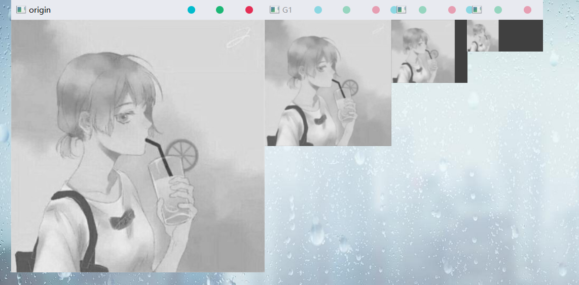
下采样

res = cv2.pyrDown(img)

示例代码：

import cv2
import numpy as np

'''读取图像'''
img = cv2.imread("../001.jpg", cv2.IMREAD_GRAYSCALE)
cv2.imshow("origin", img)

'''下采样'''
G1 = cv2.pyrDown(img)
G2 = cv2.pyrDown(G1)
G3 = cv2.pyrDown(G2)
cv2.imshow("G1", G1)
cv2.imshow("G2", G2)
cv2.imshow("G3", G3)

'''等待、关闭图像'''
cv2.waitKey(0)
cv2.destroyAllWindows()

效果：

---

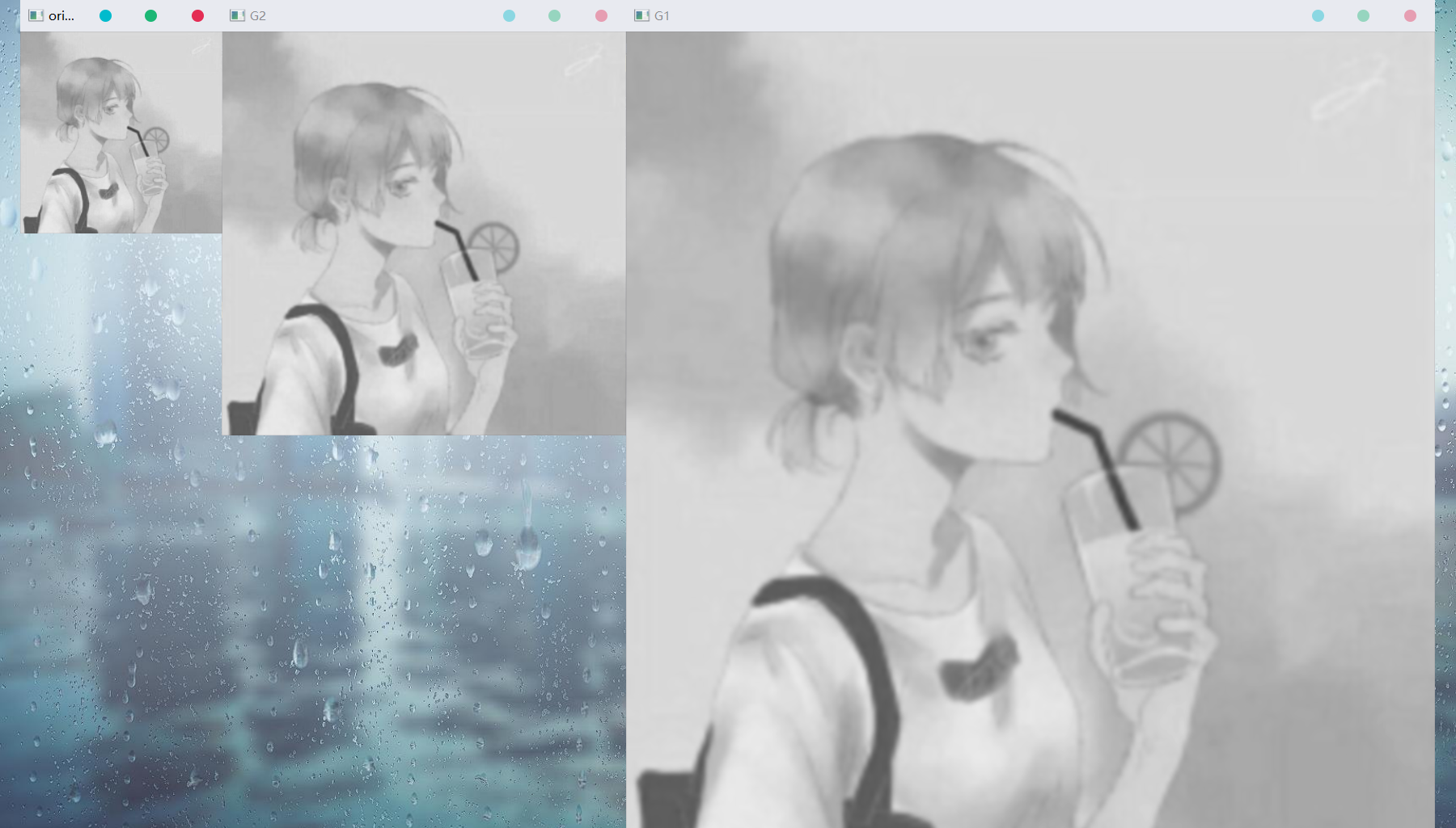
上采样

res = cv2.pyrUp(img)

示例代码：

import cv2
import numpy as np

'''读取图像'''
G3 = cv2.imread("../001.jpg", cv2.IMREAD_GRAYSCALE)
rows, cols = G3.shape[:2]
G3 = cv2.resize(G3, (rows // 2, cols // 2))
cv2.imshow("origin", G3)

'''上采样'''
G2 = cv2.pyrUp(G3)
G1 = cv2.pyrUp(G2)
cv2.imshow("G2", G2)
cv2.imshow("G1", G1)

'''等待、关闭图像'''
cv2.waitKey(0)
cv2.destroyAllWindows()

效果：

---

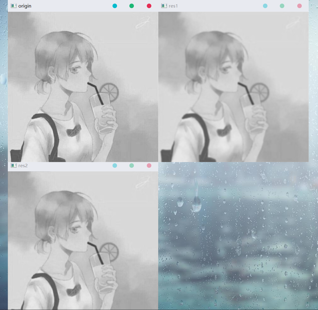
上、下采样的可逆性研究

上、下采样并非互逆操作，不论是先上采样再下采样、还是先下采样再上采样，图像的清晰度都会降低，都无法恢复原有图像

示例代码：

import cv2
import numpy as np

'''读取图像'''
img = cv2.imread("../001.jpg", cv2.IMREAD_GRAYSCALE)
cv2.imshow("origin", img)

'''先下采样，后上采样'''
down1 = cv2.pyrDown(img)
res1 = cv2.pyrUp(down1)
cv2.imshow("res1", res1)

'''先上采样，后下采样'''
up2 = cv2.pyrUp(img)
res2 = cv2.pyrDown(up2)
cv2.imshow("res2", res2)

'''等待、关闭图像'''
cv2.waitKey(0)
cv2.destroyAllWindows()

效果：

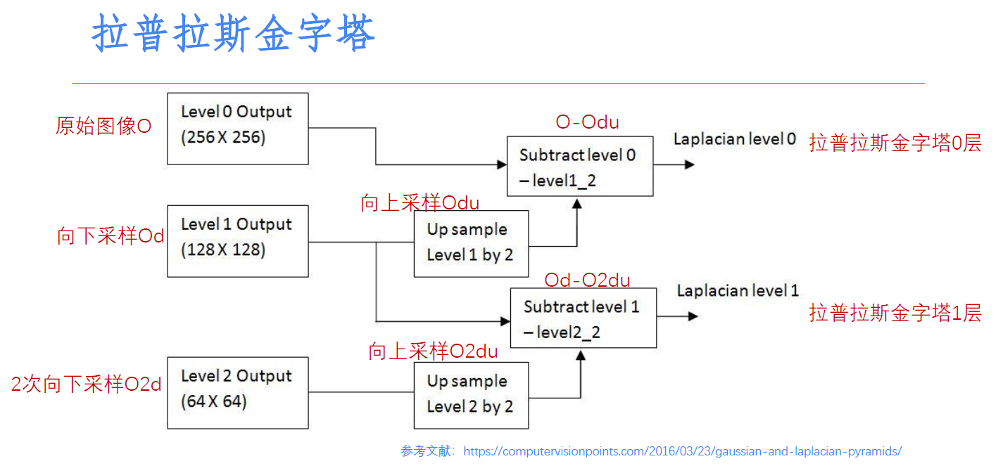
2、拉普拉斯金字塔

拉普拉斯金字塔

拉普拉斯金字塔定义在高斯金字塔的基础之上：$$\begin{array}{rl}& L_i=G_i-\text{Pyrup}(\text{PyrDown}(G_i))\\ & \\ & 其中，\{\begin{array}{ll}{G}_i& 原始图像\\ & \\ L_i& 拉普拉斯金字塔图像\end{array}\end{array}$$

拉普拉斯金字塔的结构示意如下：


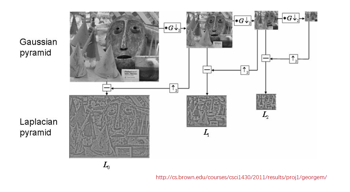
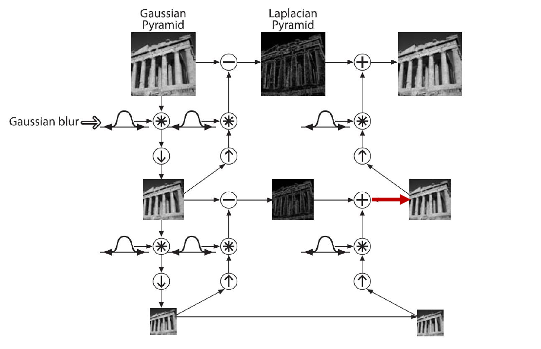
通过拉普拉斯金字塔进行计算，是可以得到原始图像的：

---

构建拉普拉斯金字塔

o
od = cv2.pyrDown(o)
odu = cv2.pyrUp(od)
l = o - odu

o1 = od
o1d = cv2.pyrDown(o1)
o1du = cv2.pyrUp(o1d)
l1 = o1 - o1du

......

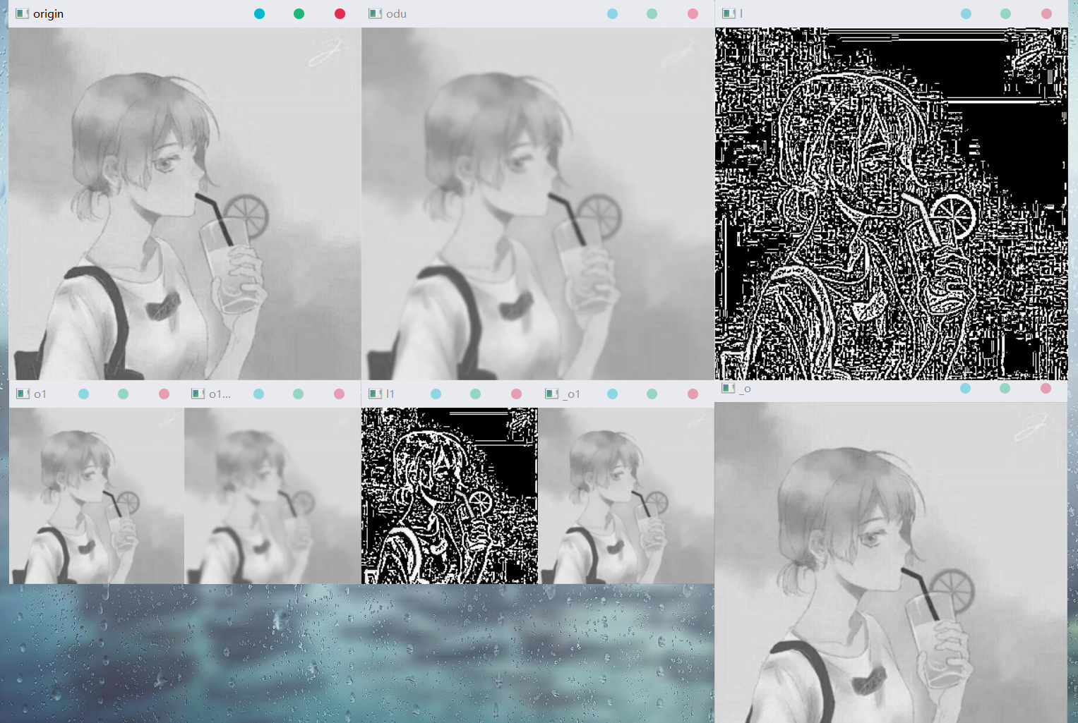
示例代码：

import cv2
import numpy as np

'''读取图像'''
o = cv2.imread("../001.jpg", cv2.IMREAD_GRAYSCALE)
cv2.imshow("origin", o)

'''构建两层拉普拉斯金字塔'''
od = cv2.pyrDown(o)
odu = cv2.pyrUp(od)
l = o - odu
cv2.imshow("odu", odu)
cv2.imshow("l", l)

o1 = od
o1d = cv2.pyrDown(o1)
o1du = cv2.pyrUp(o1d)
l1 = o1 - o1du
cv2.imshow("o1", o1)
cv2.imshow("o1du", o1du)
cv2.imshow("l1", l1)

'''根据拉普拉斯金字塔还原图像'''
_od = cv2.pyrDown(o)
_o1d = cv2.pyrDown(_od)
_o = cv2.pyrUp(_od) + l
_o1 = cv2.pyrUp(_o1d) + l1
cv2.imshow("_o", _o)
cv2.imshow("_o1", _o1)

'''等待、关闭图像'''
cv2.waitKey(0)
cv2.destroyAllWindows()

效果：

十二、图像轮廓

轮廓

边缘检测能够测出边缘，但边缘是不连续的；将边缘连接为一个整体，构成轮廓。

注意点：

• 计算轮廓的对象需为二值图像，因此需要预先进行阈值分割或者边缘检测处理
• 绘制轮廓（drawCountours）会更改原始图像，因此在绘制轮廓前，需要对原图像进行拷贝（copy）
• 在OpenCV中，黑色为背景色，白色为前景色，因此对象必须为白色，背景必须为黑色

查找轮廓

'''
返回值：
	contours							轮廓信息
	hierarchy							图像的拓扑信息（轮廓层次）
参数：
	img_bin								要操作的二值图像
	mode								轮廓的检索模式
		- cv2.RETR_EXTERNEL					只检测外轮廓
		- cv2.RETR_LIST						检测的轮廓不建立等级关系
		- cv2.RETR_CCOMP					建立两个等级的轮廓
											上面的一层为外边界
											里面的一层为内控的边界信息（若内控内还有一个连通物体，则该物体的边界也在顶层）
		★ cv2.RETR_TREE（常用）				建立一个等级树结构的轮廓
	method								轮廓的近似方法
		- cv2.CHAIN_APPROX_NONE				存储所有的轮廓点，相邻的两个点的像素位置差不超过1
											即max(abs(x1-x2), abs(y1-y2)) == 1
		- cv2.CHAIN_APPROX_SIMPLE			压缩水平方向、垂直方向、对角线方向的元素，只保留该方向的坐标终点
											例如一个矩形轮廓只要用4个点来保存轮廓信息
		- cv2.CHAIN_APPROX_TC89_L1			使用teh-Chinl chain近似算法
		- cv2.CHAIN_APPROX_TC89_KCOS		使用teh-Chinl chain近似算法
'''
contours, hiearchy = cv2.findCountours(img_bin, mode, method)

绘制轮廓

'''
contours		根据findContours计算得到的边界信息
contourIdx		需要绘制的边界索引（全部绘制则设置为-1）
color			绘制线条的颜色（BGR）
thickness		绘制线条的粗细
'''
res = cv2.drawContours(img_copy, contours, contourIdx, color[, thickness])

'''其实res和img_copy引用了同一张图像，因此我更倾向于写为以下形式'''
res = cv2.drawContours(res, contours, contourIdx, color[, thickness])

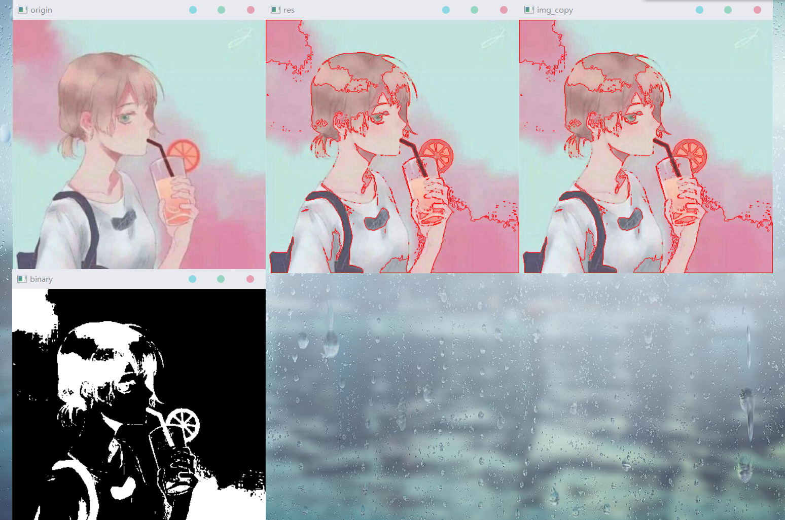
示例代码：

import cv2
import numpy as np

'''读取图像'''
img = cv2.imread("001.jpg")
rows, cols = img.shape[:2]
cv2.imshow("origin", img)

'''二值化处理'''
img_gray = cv2.cvtColor(img, cv2.COLOR_BGR2GRAY)
_, img_bin = cv2.threshold(img_gray, 180, 255, cv2.THRESH_BINARY_INV)
cv2.imshow("binary", img_bin)

'''查找轮廓'''
contours, hierarchy = cv2.findContours(img_bin, cv2.RETR_TREE, cv2.CHAIN_APPROX_SIMPLE)

'''绘制轮廓'''
img_copy = img.copy()
res = cv2.drawContours(img_copy, contours, -1, (0, 0, 255), 1)
cv2.imshow("res", res)
cv2.imshow("img_copy", img_copy)  # 拷贝图像在drawContours时已经被修改

'''等待、关闭图像'''
cv2.waitKey(0)
cv2.destroyAllWindows()

效果：

十三、直方图

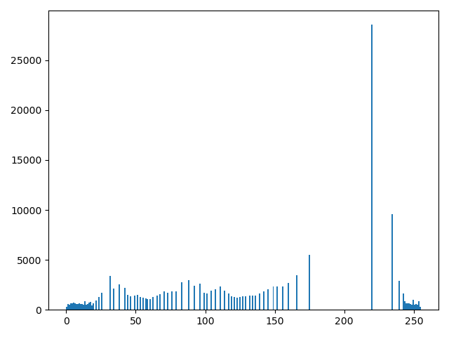
1、直方图

如下图所示，就是一个图像的直方图：

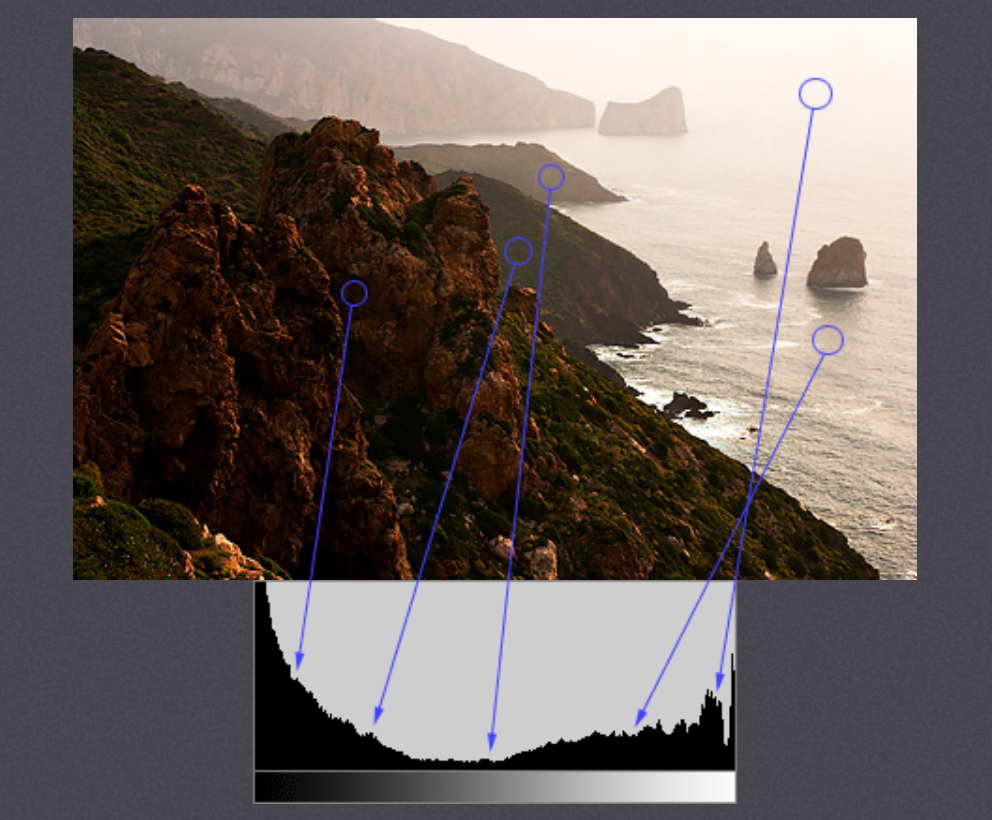
直方图的坐标定义如下：

• 横坐标：图像中各个像素点的灰度级
• 纵坐标：具有该灰度级的像素个数

类似地，还有归一化直方图：

• 横坐标：图像中各个像素点的灰度级
• 纵坐标：出现这个灰度级的概率

直方图的一些参数

• DIMS：使用参数的数量（灰度级、亮度等）
• BINS：参数子集的数目（比如灰度可以分为1-3、4-6两个级别，BINS=2）
• RANGE：统计灰度值的范围（一般为[0, 255]）

2、统计直方图

(1).Python统计直方图

img_1d = img.ravel()
plt.hist(img_1d, 256)
plt.show()

(2).OpenCV统计直方图

'''
imgs:
	图像用[]列出
channels:
	指定通道，通过[编号]指定
		绘图图像：[0]
		彩色图像：[0]——B,[1]——G,[2]——R
mask:
	统计整幅图像的直方图：设置None
	统计某一部分的直方图：设置掩码图像
histSize:
	要计算的BINS的数量，一般为[256]
ranges:
	像素值的范围，一般为[0, 255]
accumulate
	设置True/False表示是/否累积统计直方图
'''
hist = cv2.calcHist(imgs, channels, mask, histSize, ranges[, accumulate])

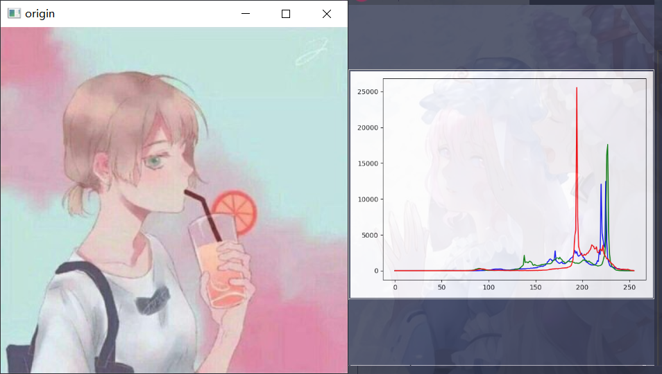
示例代码：

import cv2
import matplotlib.pyplot as plt
import numpy as np

'''读取、展示图像'''
img = cv2.imread("../001.jpg")
cv2.imshow("origin", img)

'''统计直方图'''
histB = cv2.calcHist([img], [0], None, [256], [0, 255])
histG = cv2.calcHist([img], [1], None, [256], [0, 255])
histR = cv2.calcHist([img], [2], None, [256], [0, 255])

'''绘制直方图'''
plt.plot(histB, color="b")
plt.plot(histG, color="g")
plt.plot(histR, color="r")
plt.show()

'''等待、关闭图像'''
cv2.waitKey(0)
cv2.destroyAllWindows()

效果：

3、掩膜处理

(1).掩膜构建直方图

生成掩膜图像

mask = np.zeros(img.shape, np.uint8)
mask[200:400, 200:400] = 255

示例代码：

import cv2
import matplotlib.pyplot as plt
import numpy as np

'''读取、展示图像'''
img = cv2.imread("../001.jpg", cv2.IMREAD_GRAYSCALE)
cv2.imshow("origin", img)

'''生成掩膜图像'''
mask = np.zeros(img.shape, np.uint8)
mask[200:400, 200:400] = 255

'''统计直方图'''
histG = cv2.calcHist([img], [0], None, [256], [0, 255])
histM = cv2.calcHist([img], [0], mask, [256], [0, 255])

'''绘制直方图'''
plt.plot(histG, color="g")
plt.plot(histM, color="r")
plt.show()

'''等待、关闭图像'''
cv2.waitKey(0)
cv2.destroyAllWindows()

效果：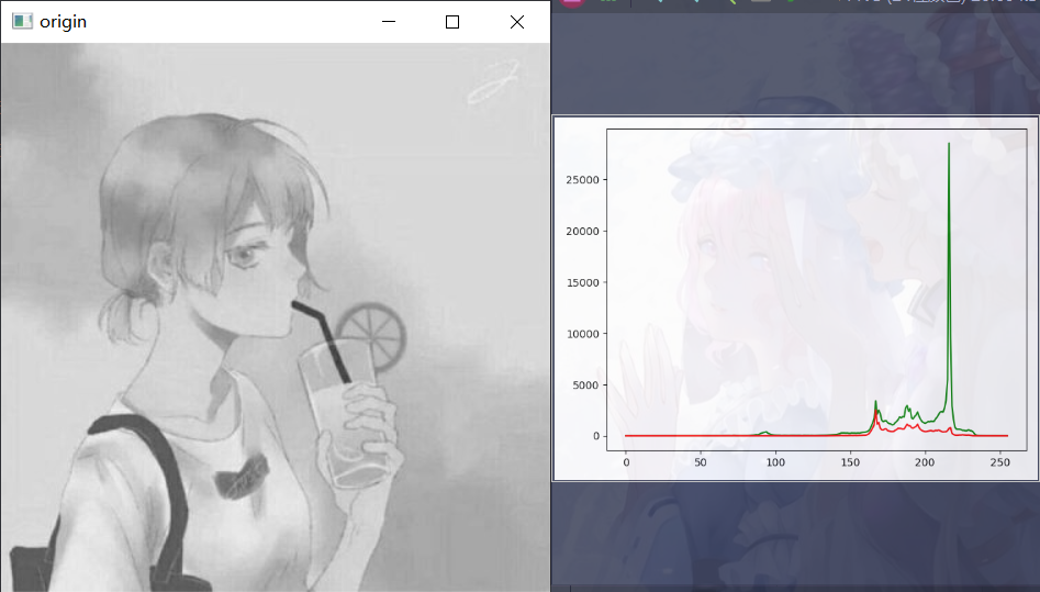

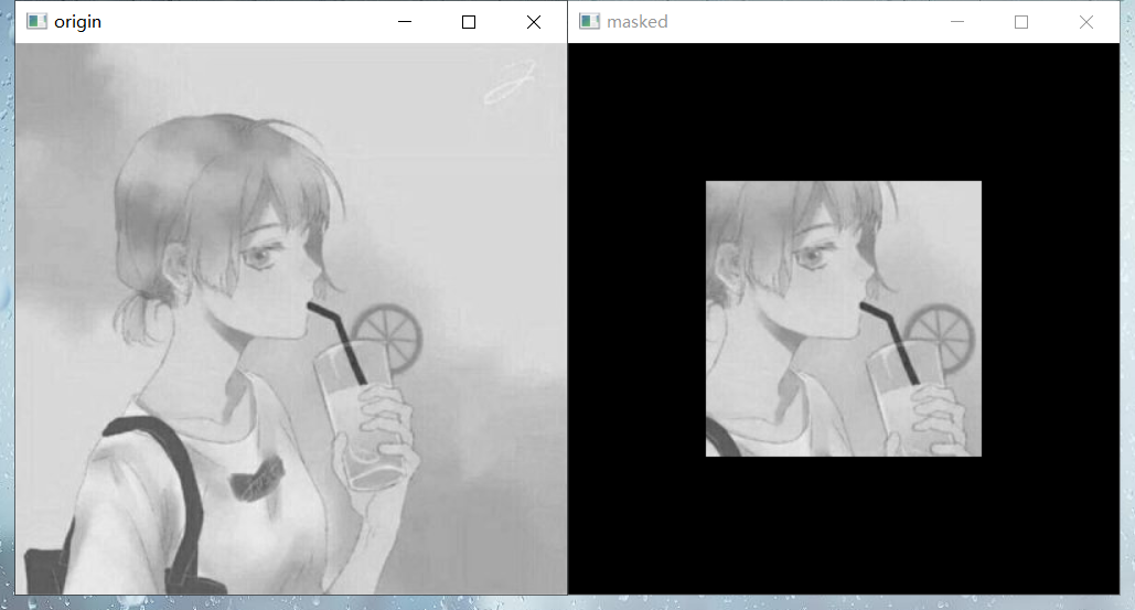
(2).掩膜处理

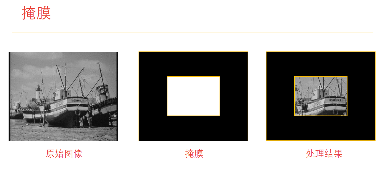
掩膜处理其实就是将原始图像和掩膜图像进行按位与操作

img_masked = cv2.bitwise_and(img, mask)

示例代码：

import cv2
import matplotlib.pyplot as plt
import numpy as np

'''读取、展示图像'''
img = cv2.imread("../001.jpg", cv2.IMREAD_GRAYSCALE)
cv2.imshow("origin", img)

'''生成掩膜图像'''
mask = np.zeros(img.shape, np.uint8)
mask[100:300, 100:300] = 255

'''掩膜处理'''
img_masked = cv2.bitwise_and(img, mask)
cv2.imshow("masked", img_masked)

'''等待、关闭图像'''
cv2.waitKey(0)
cv2.destroyAllWindows()

效果：

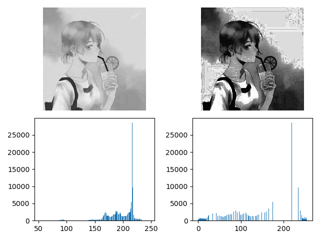
4、直方图均衡化

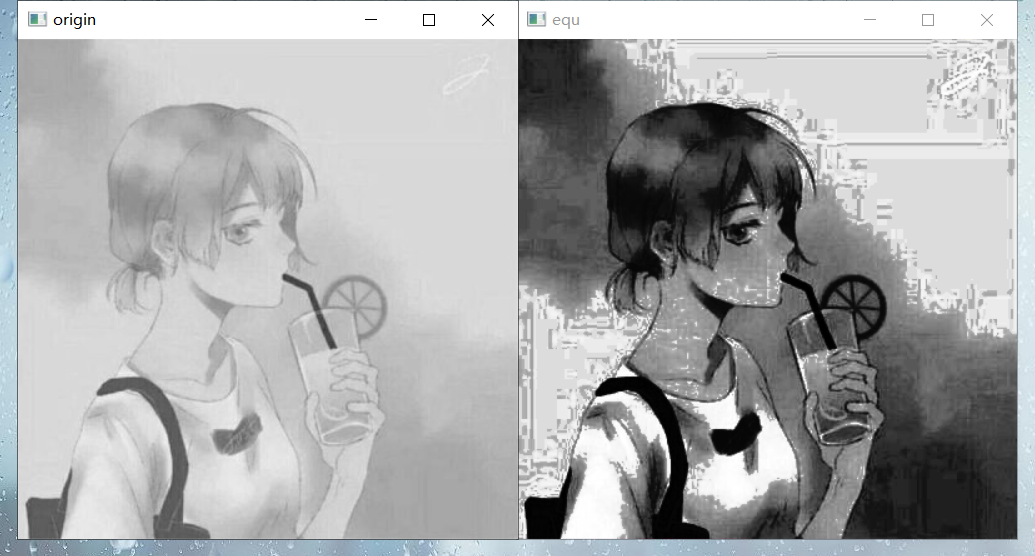
直方图均衡化

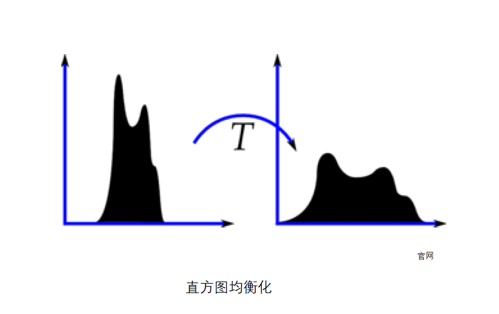
通过直方图的均衡化，可以将较亮/较暗的图像处理为比较正常的图像：

---

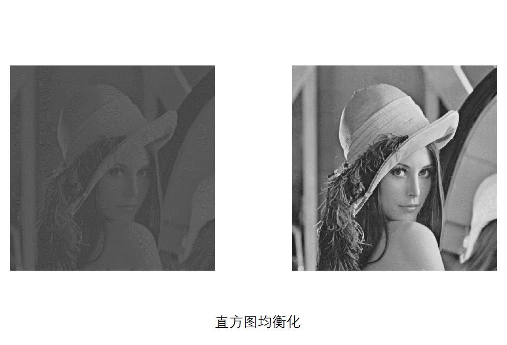
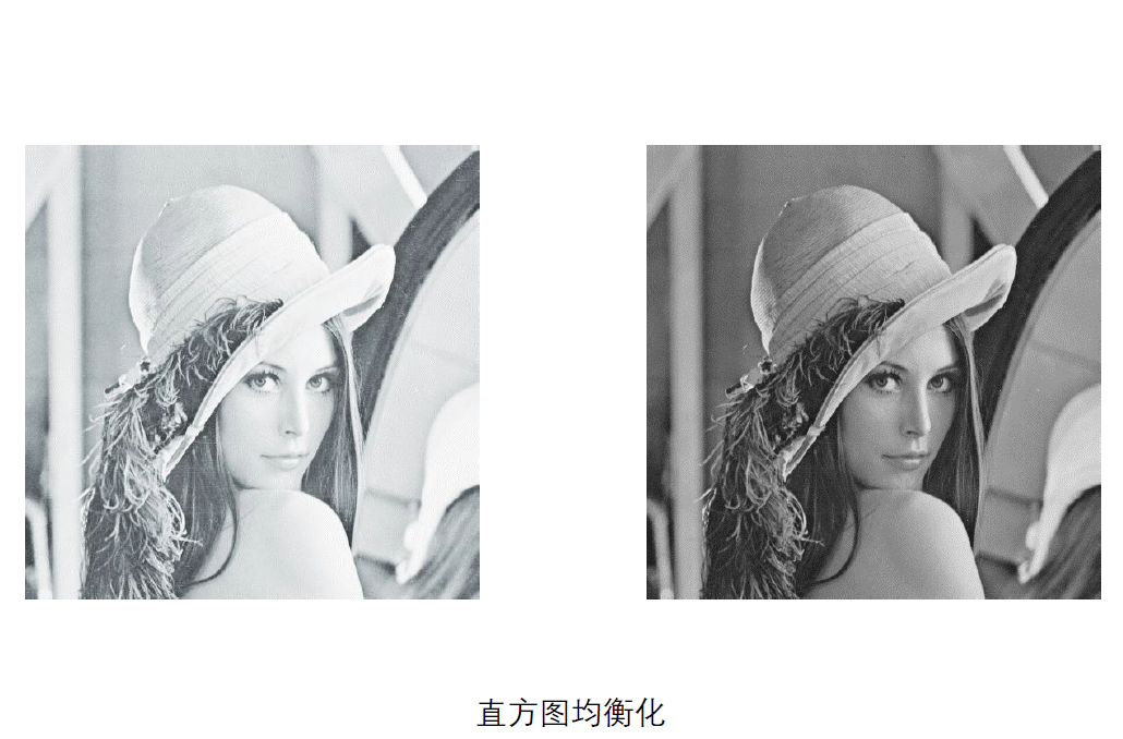
直方图均衡化的图像特征

• 前提：占有全部可能的灰度级并且均匀分布
• 结论：具有高对比度和多变的灰度色调
• 外观：图像细节丰富，质量更高

---

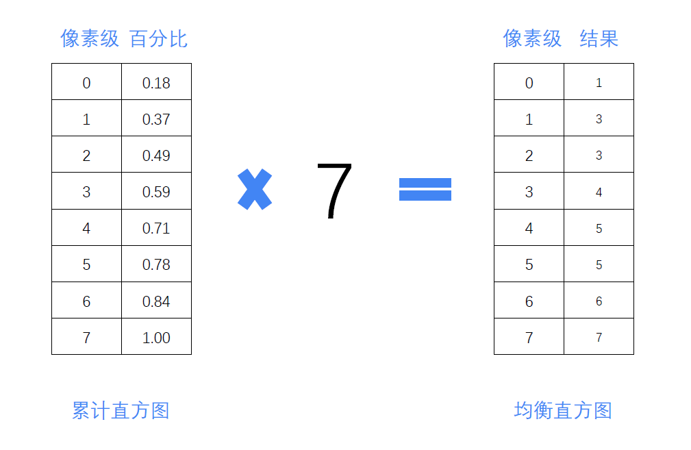
均衡化步骤

1. 计算累计直方图
2. 将累计直方图进行区间转换
3. 在累积直方图中，概率相近的原始值，会被处理为相同的值（人眼处理）

---

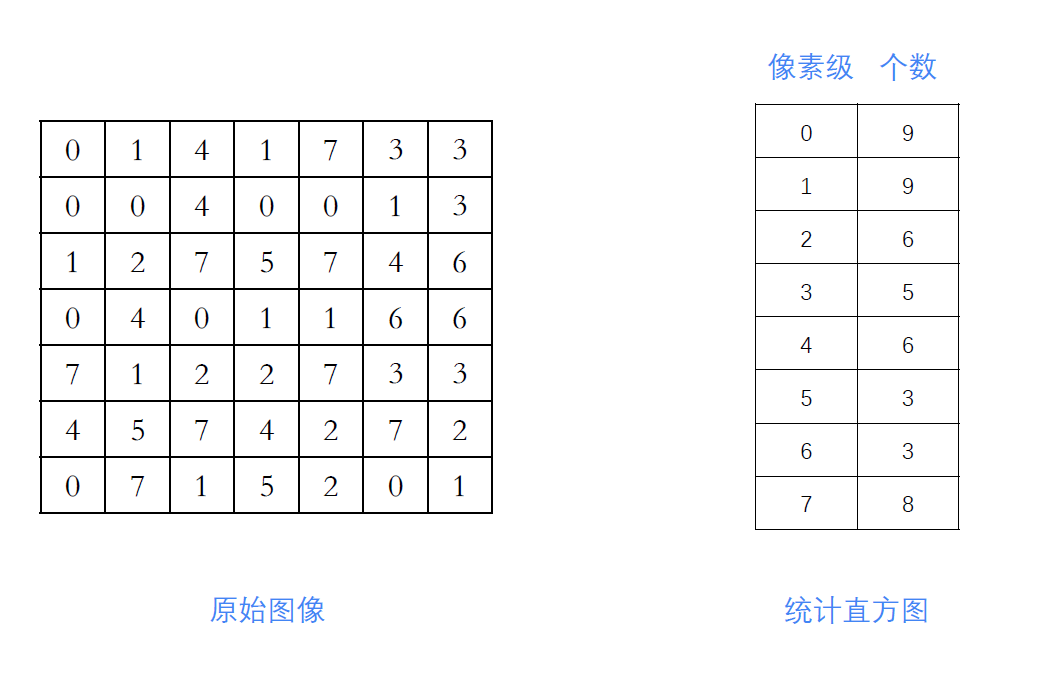
具体步骤

原始图像→统计直方图→归一化直方图→累计直方图→均衡直方图

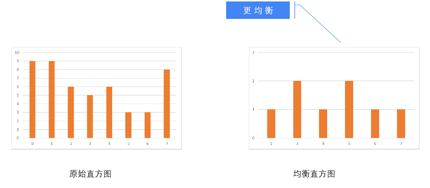
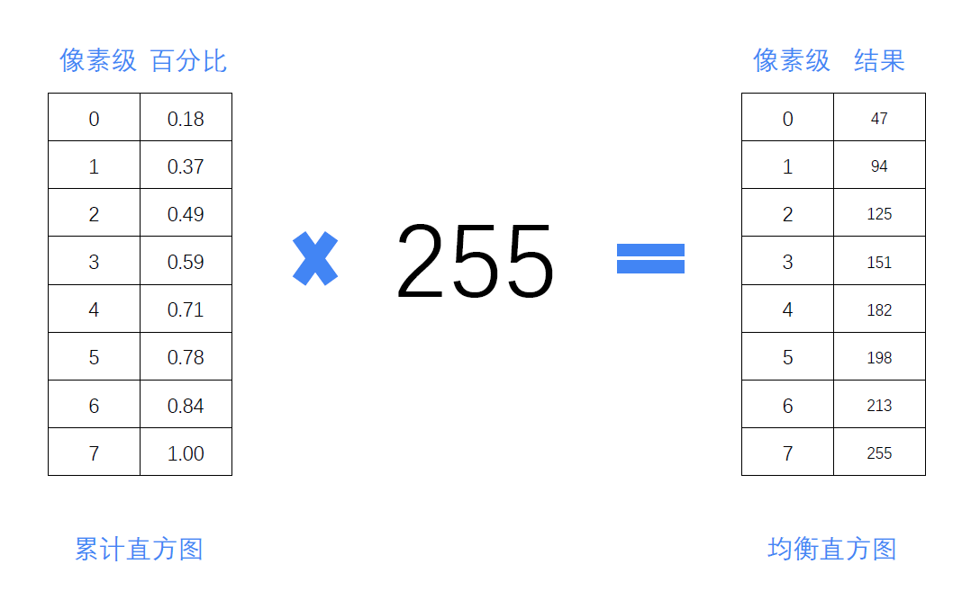
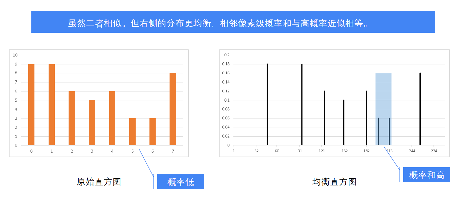
上述案例中，*255的例子虽然198和213的部分在整个直方图上看起来不均匀，但是由于这两块的值比较接近、颜色相近，肉眼会将它们视为一种颜色，因此统计直方图可以将这两部分视为一块，概率和放在这里在整个直方图上还是比较均匀的（简单来说，就是密集的地方概率小、稀疏的地方概率大）。

---

应用场景：

• 医疗图像处理
• 车牌识别
• 人脸识别

---

直方图均衡化

res = cv2.equalizeHist(img)

示例代码：

import cv2
import matplotlib.pyplot as plt
import numpy as np

'''读取、展示图像'''
img = cv2.imread("../001.jpg", cv2.IMREAD_GRAYSCALE)
cv2.imshow("origin", img)

'''直方图均衡化'''
equ = cv2.equalizeHist(img)
cv2.imshow("equ", equ)

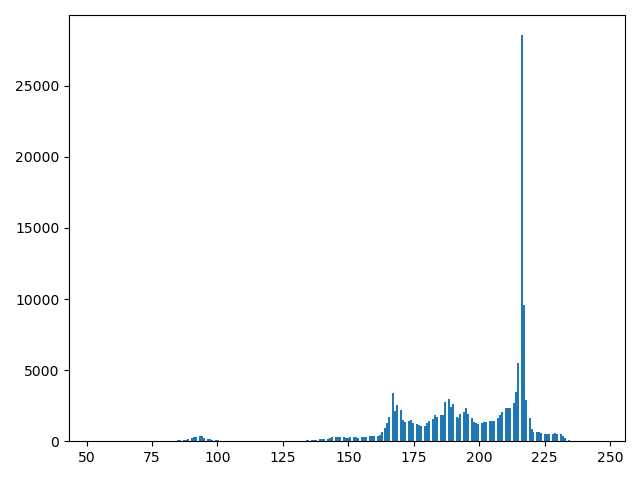
'''绘制直方图'''
plt.hist(img.ravel(), 256)
plt.figure()
plt.hist(equ.ravel(), 256)
plt.show()

'''等待、关闭图像'''
cv2.waitKey(0)
cv2.destroyAllWindows()

效果：

合并绘图

'''
分nrows行，ncols列，绘制第plot_number个

特殊地，当每一个参数都小于10时，可以直接将三个数字写在一起（如：subplot(234)）
'''
subplot(nrows, ncols, plot_number)

plt绘图

'''
彩色图像：
	cv2默认使用BGR通道
	plt默认使用RGB通道
	因此cv2读入的图像需要先进行通道调整才能用plt进行展示
灰度图像：
	设置参数cmap=plt.cm.gray
'''
plt.imshow(img, camp=XXX)

示例代码：

import cv2
import matplotlib.pyplot as plt
import numpy as np

'''读取、展示图像'''
img = cv2.imread("../001.jpg", cv2.IMREAD_GRAYSCALE)
cv2.imshow("origin", img)

'''直方图均衡化'''
equ = cv2.equalizeHist(img)
cv2.imshow("equ", equ)

'''绘制直方图'''
plt.subplot(221)
plt.imshow(img, cmap=plt.cm.gray)
plt.axis('off')

plt.subplot(222)
plt.imshow(equ, cmap=plt.cm.gray)
plt.axis('off')

plt.subplot(223)
plt.hist(img.ravel(), 256)

plt.subplot(224)
plt.hist(equ.ravel(), 256)

plt.show()

'''等待、关闭图像'''
cv2.waitKey(0)
cv2.destroyAllWindows()

效果：

十四、傅里叶变换

1、傅里叶变换

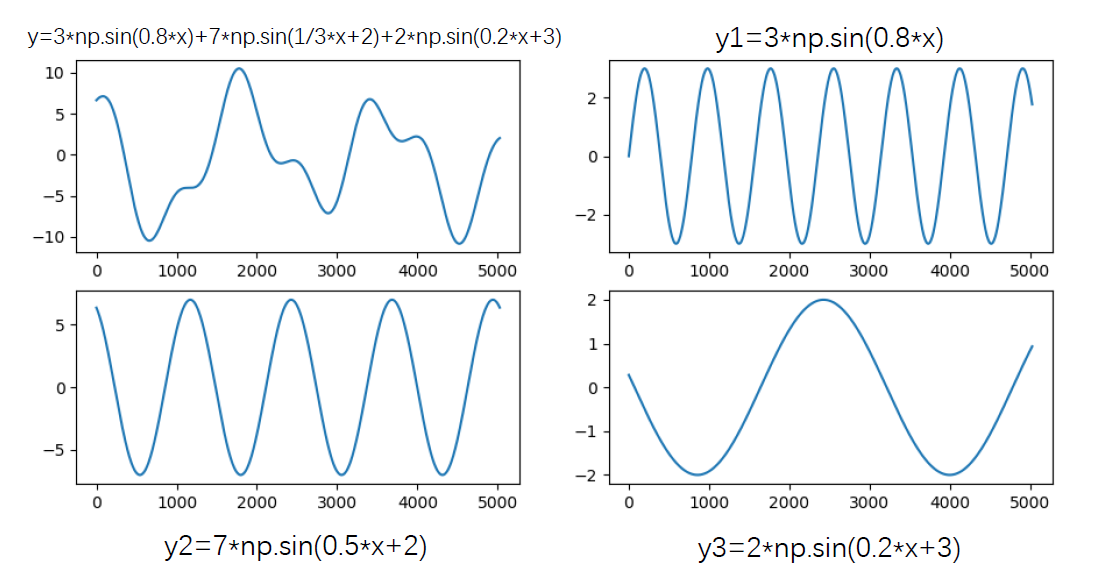
任何连续周期信号，可以由一组适当的正弦曲线组合而成。

——傅里叶

一个正弦曲线可以等价于一组[频率, 振幅, 相位]

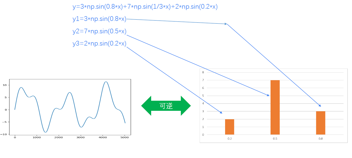
一个复杂的曲线也可以由多个正弦曲线组合而成

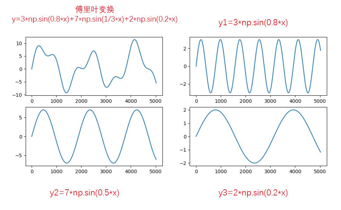
Tips：傅里叶变换是可逆的

Tips：有时候开始的时间不一样，需要使用相位

Tips：

• 傅里叶变换得到低频、高频信息，针对低频、高频处理能够实现不同的目的
• 傅里叶变换可逆，图像经过傅里叶变换、逆傅里叶变换后，能够恢复到原始图像
• 在频域对图像进行处理，会反映在逆变换的图像上

---

Numpy实现

# 实现傅里叶变换，得到复数数组
f = np.fft.fft2(img)
# 将低频移动到中心位置
f_shift = np.fft.fftshift(f)
# 将复数数组映射到0-255的像素数组
res = 20 * np.log(np.abs(f_shift))

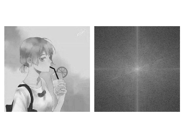
示例代码：

import cv2
import matplotlib.pyplot as plt
import numpy as np

'''读取、展示图像'''
img = cv2.imread("../001.jpg", cv2.IMREAD_GRAYSCALE)
cv2.imshow("origin", img)

'''傅里叶变换'''
f = np.fft.fft2(img)
f_shift = np.fft.fftshift(f)
res = 20 * np.log(np.abs(f_shift))

'''绘图'''
plt.subplot(121)
plt.imshow(img, cmap="gray")
plt.axis("off")

plt.subplot(122)
plt.imshow(res, cmap="gray")
plt.axis("off")

plt.show()

'''等待、关闭图像'''
cv2.waitKey(0)
cv2.destroyAllWindows()

效果：

---

OpenCV实现

# 图像类型转换
img_32 = np.float32(img)

'''
傅里叶变换
	f
		双通道
		第1个通道是结果的实数部分
		第2个通道是结果的虚数部分
	
	img_32
		要求转换为np.float32格式：np.float32(img)
	flags
		一般使用cv2.DFT_COPLEX_OUTPUT，输出一个附属阵列
'''
f = cv2.dft(img_32, cv2.DFT_COMPLEX_OUTPUT)
f_shift = np.fft.fftshift(f)

# 计算幅值（其实就是计算复数的模）
f_abs = cv2.magnitude(f_shift[:,:,0],f_shift[:,:,1])

# 区间映射
f_res = 20 * np.log(f_abs)

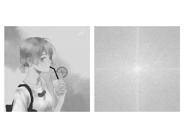
示例代码：

import cv2
import matplotlib.pyplot as plt
import numpy as np

'''读取、展示图像'''
img = cv2.imread("../001.jpg", cv2.IMREAD_GRAYSCALE)
cv2.imshow("origin", img)

'''傅里叶变换'''
img_32 = np.float32(img)
f = cv2.dft(img_32, flags=cv2.DFT_COMPLEX_OUTPUT)
f_shift = np.fft.fftshift(f)
f_abs = cv2.magnitude(f_shift[:, :, 0], f_shift[:, :, 0])
res = 20 * np.log(f_abs + 1e-9)

'''绘图'''
plt.subplot(121)
plt.imshow(img, cmap="gray")
plt.axis("off")

plt.subplot(122)
plt.imshow(res, cmap="gray")
plt.axis("off")

plt.show()

'''等待、关闭图像'''
cv2.waitKey(0)
cv2.destroyAllWindows()

效果：

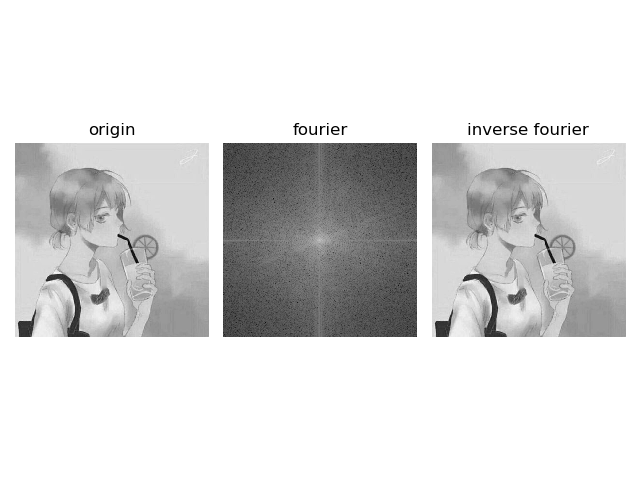
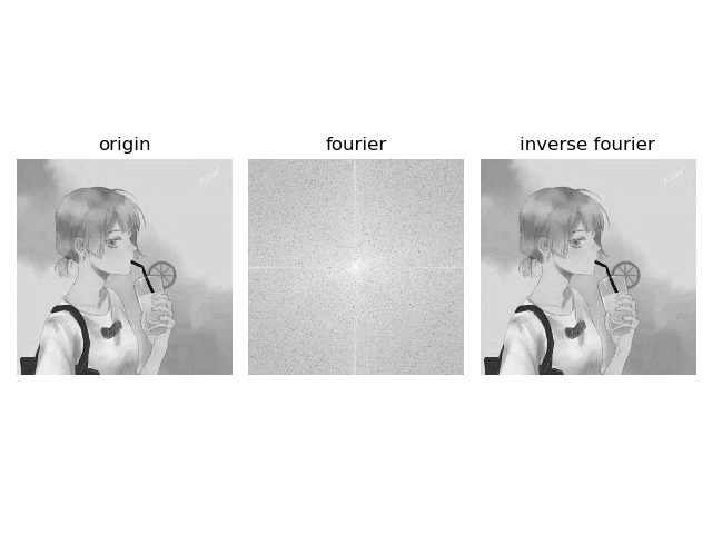
2、逆傅里叶变换

通过傅里叶变换，我们可以得到一个频谱

我们可以根据频谱对该频谱上特定的高频/低频处进行操作

通过逆傅里叶变换，我们可以把频谱还原为图像

---

Numpy实现

'''傅里叶变换'''
f = np.fft.fft2(img)
f_shift = np.fft.fftshift(f)

'''逆傅里叶变换'''
i_shift = np.fft.ifftshift(f_shift)
i = np.fft.ifft2(i_shift)
res = np.abs(i)

示例代码：

import cv2
import matplotlib.pyplot as plt
import numpy as np

'''读取、展示图像'''
img = cv2.imread("../001.jpg", cv2.IMREAD_GRAYSCALE)
cv2.imshow("origin", img)

'''傅里叶变换'''
f = np.fft.fft2(img)
f_shift = np.fft.fftshift(f)
res_f = 20 * np.log(np.abs(f_shift))

'''逆傅里叶变换'''
i_shift = np.fft.ifftshift(f_shift)
i = np.fft.ifft2(i_shift)
res_i = np.abs(i)

'''绘图'''
plt.subplot(131)
plt.imshow(img, cmap="gray")
plt.title("origin")
plt.axis("off")

plt.subplot(132)
plt.imshow(res_f, cmap="gray")
plt.title("fourier")
plt.axis("off")

plt.subplot(133)
plt.imshow(res_i, cmap="gray")
plt.title("inverse fourier")
plt.axis("off")

plt.show()

'''等待、关闭图像'''
cv2.waitKey(0)
cv2.destroyAllWindows()

效果：

---

OpenCV实现

'''傅里叶变换'''
img_32 = np.float32(img)
f = cv2.dft(img_32, cv2.DFT_COMPLEX_OUTPUT)
f_shift = np.fft.fftshift(f)

'''逆傅里叶变换'''
i_shift = np.fft.ifftshift(f_shift)
i = cv2.idft(i_shift)
res_i = cv2.magnitude(i[:, :, 0], i[:, :, 1])

示例代码：

import cv2
import matplotlib.pyplot as plt
import numpy as np

'''读取、展示图像'''
img = cv2.imread("../001.jpg", cv2.IMREAD_GRAYSCALE)
cv2.imshow("origin", img)

'''傅里叶变换'''
img_32 = np.float32(img)
f = cv2.dft(img_32, flags=cv2.DFT_COMPLEX_OUTPUT)
f_shift = np.fft.fftshift(f)
f_abs = cv2.magnitude(f_shift[:, :, 0], f_shift[:, :, 0])
f_res = 20 * np.log(f_abs + 1e-9)

'''逆傅里叶变换'''
i_shift = np.fft.ifftshift(f_shift)
i = cv2.idft(i_shift)
i_res = cv2.magnitude(i[:, :, 0], i[:, :, 1])

'''绘图'''
plt.subplot(131)
plt.imshow(img, cmap="gray")
plt.title("origin")
plt.axis("off")

plt.subplot(132)
plt.imshow(f_res, cmap="gray")
plt.title("fourier")
plt.axis("off")

plt.subplot(133)
plt.imshow(i_res, cmap="gray")
plt.title("inverse fourier")
plt.axis("off")

plt.show()

'''等待、关闭图像'''
cv2.waitKey(0)
cv2.destroyAllWindows()

效果：

3、滤波

(1).滤波

低频对应图像内变化缓慢的灰度分量（如：大草原的图像中，颜色趋于一致的草原）

高频对应图像内变化越来越快的灰度分量，由灰度的尖锐过度造成（如：大草原的图像中，狮子的边缘等信息）

滤波

• 通过/拒绝一定频率的分量
• 通过低频的滤波器称为低通滤波器
  低通滤波器将会模糊一些图像
• 通过高频的滤波器称为高通滤波器
  高通滤波器将会增强图像中尖锐的细节，但会导致图像的对比度降低

频域滤波

先进行傅里叶变换得到图像的高频/低频信息，对其进行处理，再进行逆傅里叶变换还原为图像，以达到特殊目的：

• 图像增强
• 图像去噪
• 边缘检测
• 特征提取
• 压缩
• 加密
• ……

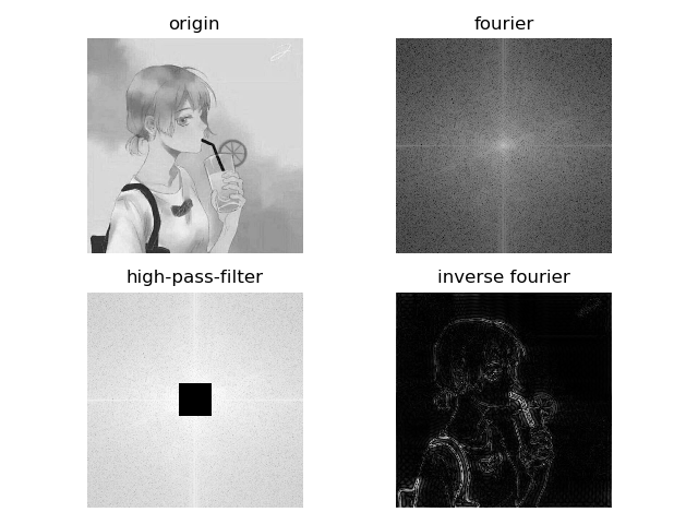
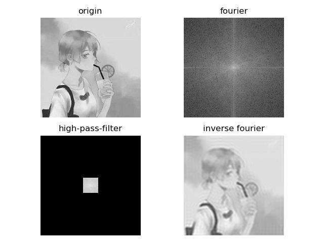
(2).高通滤波

高通滤波

rows, cols = img.shape
crow, ccol = rows // 2, cols // 2
f_shift[crow - 30:crow + 30, ccol - 30:ccol + 30] = 0

---

示例代码（Numpy）：

import cv2
import matplotlib.pyplot as plt
import numpy as np

'''读取、展示图像'''
img = cv2.imread("../001.jpg", cv2.IMREAD_GRAYSCALE)
cv2.imshow("origin", img)

'''傅里叶变换'''
f = np.fft.fft2(img)
f_shift = np.fft.fftshift(f)
res_f = 20 * np.log(np.abs(f_shift))

'''高通滤波'''
rows, cols = img.shape
crow, ccol = rows // 2, cols // 2
f_shift[crow - 30:crow + 30, ccol - 30:ccol + 30] = 0

res_f2 = 20 * np.log(np.abs(f_shift) + 1e-9)

'''逆傅里叶变换'''
i_shift = np.fft.ifftshift(f_shift)
i = np.fft.ifft2(i_shift)
res_i = np.abs(i)
res_i = np.uint8(res_i / res_i.max() * 256)

cv2.imshow("res", res_i)

'''绘图'''
plt.subplot(221)
plt.imshow(img, cmap="gray")
plt.title("origin")
plt.axis("off")

plt.subplot(222)
plt.imshow(res_f, cmap="gray")
plt.title("fourier")
plt.axis("off")

plt.subplot(223)
plt.imshow(res_f2, cmap="gray")
plt.title("high-pass-filter")
plt.axis("off")

plt.subplot(224)
plt.imshow(res_i, cmap="gray")
plt.title("inverse fourier")
plt.axis("off")

plt.show()

'''等待、关闭图像'''
cv2.waitKey(0)
cv2.destroyAllWindows()

效果：

---

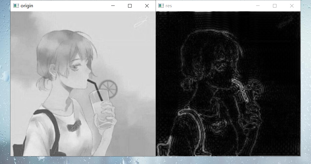
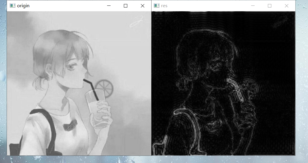
示例代码（OpenCV）：

import cv2
import matplotlib.pyplot as plt
import numpy as np

'''读取、展示图像'''
img = cv2.imread("../001.jpg", cv2.IMREAD_GRAYSCALE)
cv2.imshow("origin", img)

'''傅里叶变换'''
img_32 = np.float32(img)
f = cv2.dft(img_32, flags=cv2.DFT_COMPLEX_OUTPUT)
f_shift = np.fft.fftshift(f)
f_abs = cv2.magnitude(f_shift[:, :, 0], f_shift[:, :, 1])
res_f = 20 * np.log(f_abs)

'''高通滤波'''
rows, cols = img.shape
crow, ccol = rows // 2, cols // 2
f_shift[crow - 30:crow + 30, ccol - 30:ccol + 30, :] = 0
f_abs2 = cv2.magnitude(f_shift[:, :, 0], f_shift[:, :, 1])

res_f2 = 20 * np.log(f_abs2 + 1e-9)

'''逆傅里叶变换'''
i_shift = np.fft.ifftshift(f_shift)
i = cv2.idft(i_shift)
res_i = cv2.magnitude(i[:, :, 0], i[:, :, 1])
res_i = np.uint8(res_i / res_i.max() * 256)

cv2.imshow("res", res_i)

'''绘图'''
plt.subplot(221)
plt.imshow(img, cmap="gray")
plt.title("origin")
plt.axis("off")

plt.subplot(222)
plt.imshow(res_f, cmap="gray")
plt.title("fourier")
plt.axis("off")

plt.subplot(223)
plt.imshow(res_f2, cmap="gray")
plt.title("high-pass-filter")
plt.axis("off")

plt.subplot(224)
plt.imshow(res_i, cmap="gray")
plt.title("inverse fourier")
plt.axis("off")

plt.show()

'''等待、关闭图像'''
cv2.waitKey(0)
cv2.destroyAllWindows()

效果：

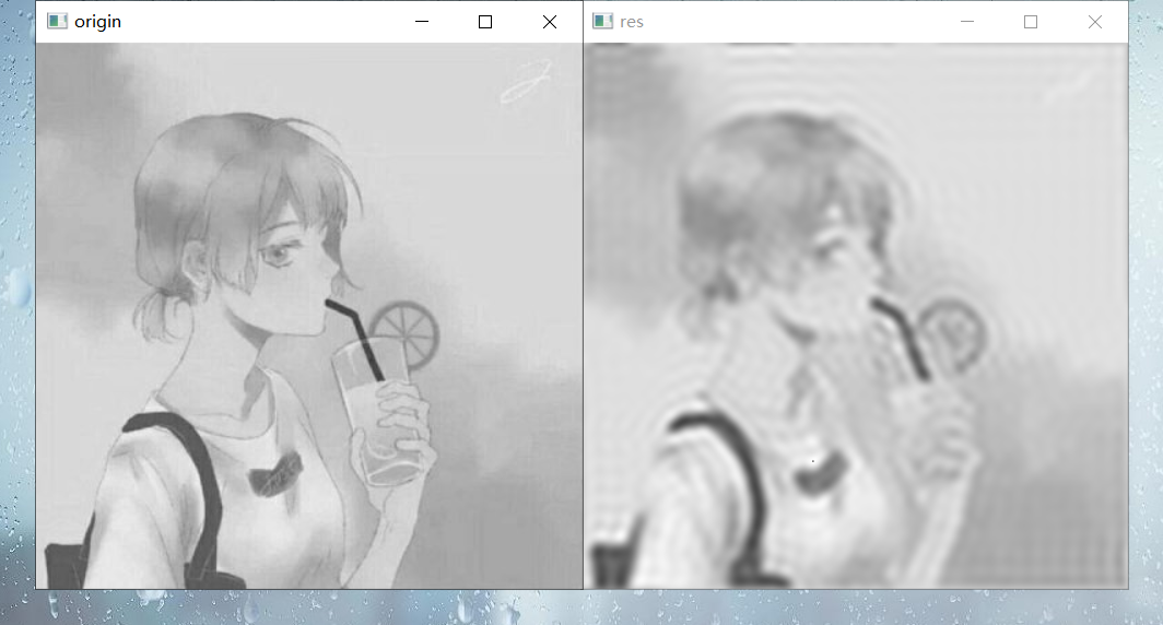
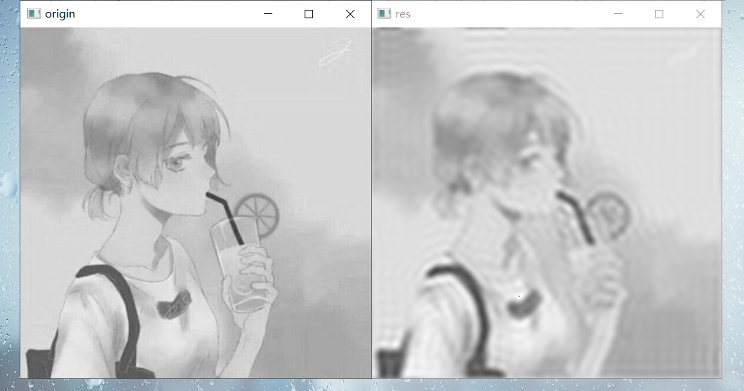
(3).低通滤波

低通滤波

rows, cols = img.shape
crow, ccol = rows // 2, cols // 2
mask = np.zeros((rows, cols, 2), np.uint8)
mask[crow - 30:crow + 30, ccol - 30:ccol + 30] = 1
f_shift *= mask

---

示例代码（Numpy）：

import cv2
import matplotlib.pyplot as plt
import numpy as np

'''读取、展示图像'''
img = cv2.imread("../001.jpg", cv2.IMREAD_GRAYSCALE)
cv2.imshow("origin", img)

'''傅里叶变换'''
f = np.fft.fft2(img)
f_shift = np.fft.fftshift(f)
res_f = 20 * np.log(np.abs(f_shift))

'''低通滤波'''
rows, cols = img.shape
crow, ccol = rows // 2, cols // 2
mask = np.zeros((rows, cols), np.uint8)
mask[crow - 30:crow + 30, ccol - 30:ccol + 30] = 1
f_shift *= mask

res_f2 = 20 * np.log(np.abs(f_shift) + 1e-9)

'''逆傅里叶变换'''
i_shift = np.fft.ifftshift(f_shift)
i = np.fft.ifft2(i_shift)
res_i = np.abs(i)
res_i = np.uint8(res_i / res_i.max() * 256)

cv2.imshow("res", res_i)

'''绘图'''
plt.subplot(221)
plt.imshow(img, cmap="gray")
plt.title("origin")
plt.axis("off")

plt.subplot(222)
plt.imshow(res_f, cmap="gray")
plt.title("fourier")
plt.axis("off")

plt.subplot(223)
plt.imshow(res_f2, cmap="gray")
plt.title("high-pass-filter")
plt.axis("off")

plt.subplot(224)
plt.imshow(res_i, cmap="gray")
plt.title("inverse fourier")
plt.axis("off")

plt.show()

'''等待、关闭图像'''
cv2.waitKey(0)
cv2.destroyAllWindows()

效果：

---

示例代码（OpenCV）：

import cv2
import matplotlib.pyplot as plt
import numpy as np

'''读取、展示图像'''
img = cv2.imread("../001.jpg", cv2.IMREAD_GRAYSCALE)
cv2.imshow("origin", img)

'''傅里叶变换'''
img_32 = np.float32(img)
f = cv2.dft(img_32, flags=cv2.DFT_COMPLEX_OUTPUT)
f_shift = np.fft.fftshift(f)
f_abs = cv2.magnitude(f_shift[:, :, 0], f_shift[:, :, 1])
res_f = 20 * np.log(f_abs)

'''高通滤波'''
rows, cols = img.shape
crow, ccol = rows // 2, cols // 2
mask = np.zeros((rows, cols, 2), np.uint8)
mask[crow - 30:crow + 30, ccol - 30:ccol + 30, :] = 1
f_shift *= mask
f_abs2 = cv2.magnitude(f_shift[:, :, 0], f_shift[:, :, 1])

res_f2 = 20 * np.log(f_abs2 + 1e-9)

'''逆傅里叶变换'''
i_shift = np.fft.ifftshift(f_shift)
i = cv2.idft(i_shift)
res_i = cv2.magnitude(i[:, :, 0], i[:, :, 1])
res_i = np.uint8(res_i / res_i.max() * 256)

cv2.imshow("res", res_i)

'''绘图'''
plt.subplot(221)
plt.imshow(img, cmap="gray")
plt.title("origin")
plt.axis("off")

plt.subplot(222)
plt.imshow(res_f, cmap="gray")
plt.title("fourier")
plt.axis("off")

plt.subplot(223)
plt.imshow(res_f2, cmap="gray")
plt.title("high-pass-filter")
plt.axis("off")

plt.subplot(224)
plt.imshow(res_i, cmap="gray")
plt.title("inverse fourier")
plt.axis("off")

plt.show()

'''等待、关闭图像'''
cv2.waitKey(0)
cv2.destroyAllWindows()

效果：