Linear Regression using Scikit-Learn

Scikit-Learn

scikit-learn是一款开源的，非常有用的机器学习工具集。

在利用梯度下降进行线性回归的部分，我们会使用sklearn.linear_model.SGDRegressor线性回归模型，这个模型类似我们之前实现的线性回归模型，并使用sklearn.preprocessing.StandardScaler对模型进行z-score标准化，在这里被称为standard score标准化。

这两个都是类，使用的时候需要先构造一个实例。

class sklearn.linear_model.SGDRegressor

Parameters:

• loss:str, default=’squared_error’

  使用的损失函数. 可能的取值为 ‘squared_error’, ‘huber’, ‘epsilon_insensitive’, or ‘squared_epsilon_insensitive’

  ‘squared_error’ 使用普通的最小二乘法. ‘huber’ 改进了‘squared_error’ ，通过从平方loss改为线性loss，使得不需要考虑如何将异常值（outlier）纠正。‘epsilon_insensitive’ 忽略小于$epsilon$的误差，这也是SVR中使用的损失函数。 ‘squared_epsilon_insensitive’ 也类似，不过使用平方损失，失去了对$ϵ$的容错（past a tolerance of epsilon）。

  More details about the losses formulas can be found in the User Guide.

• penalty:{‘l2’, ‘l1’, ‘elasticnet’, None}, default=’l2’

  The penalty (aka regularization term) to be used. Defaults to ‘l2’ which is the standard regularizer for linear SVM models. ‘l1’ and ‘elasticnet’ might bring sparsity to the model (feature selection) not achievable with ‘l2’. No penalty is added when set to None.

• alpha:float, default=0.0001

  Constant that multiplies the regularization term. The higher the value, the stronger the regularization. Also used to compute the learning rate when set to learning_rate is set to ‘optimal’.

• l1_ratio:float, default=0.15

  The Elastic Net mixing parameter, with 0 <= l1_ratio <= 1. l1_ratio=0 corresponds to L2 penalty, l1_ratio=1 to L1. Only used if penalty is ‘elasticnet’.

• fit_intercept:bool, default=True

  Whether the intercept should be estimated or not. If False, the data is assumed to be already centered.

• max_iter:int, default=1000

  The maximum number of passes over the training data (aka epochs). It only impacts the behavior in the fit method, and not the partial_fit method.New in version 0.19.

• tol:float or None, default=1e-3

  The stopping criterion. If it is not None, training will stop when (loss > best_loss - tol) for n_iter_no_change consecutive epochs. Convergence is checked against the training loss or the validation loss depending on the early_stopping parameter.New in version 0.19.

• shuffle:bool, default=True

  Whether or not the training data should be shuffled after each epoch.

• verbose:int, default=0

  The verbosity level.

• epsilon:float, default=0.1

  Epsilon in the epsilon-insensitive loss functions; only if loss is ‘huber’, ‘epsilon_insensitive’, or ‘squared_epsilon_insensitive’. For ‘huber’, determines the threshold at which it becomes less important to get the prediction exactly right. For epsilon-insensitive, any differences between the current prediction and the correct label are ignored if they are less than this threshold.

• random_state:int, RandomState instance, default=None

  Used for shuffling the data, when shuffle is set to True. Pass an int for reproducible output across multiple function calls. See Glossary.

• learning_rate:str, default=’invscaling’

  The learning rate schedule:‘constant’: eta = eta0‘optimal’: eta = 1.0 / (alpha * (t + t0)) where t0 is chosen by a heuristic proposed by Leon Bottou.‘invscaling’: eta = eta0 / pow(t, power_t)‘adaptive’: eta = eta0, as long as the training keeps decreasing. Each time n_iter_no_change consecutive epochs fail to decrease the training loss by tol or fail to increase validation score by tol if early_stopping is True, the current learning rate is divided by 5.New in version 0.20: Added ‘adaptive’ option

• eta0:float, default=0.01

  The initial learning rate for the ‘constant’, ‘invscaling’ or ‘adaptive’ schedules. The default value is 0.01.

• power_t:float, default=0.25

  The exponent for inverse scaling learning rate.

• early_stopping:bool, default=False

  Whether to use early stopping to terminate training when validation score is not improving. If set to True, it will automatically set aside a fraction of training data as validation and terminate training when validation score returned by the score method is not improving by at least tol for n_iter_no_change consecutive epochs.New in version 0.20: Added ‘early_stopping’ option

• validation_fraction:float, default=0.1

  The proportion of training data to set aside as validation set for early stopping. Must be between 0 and 1. Only used if early_stopping is True.New in version 0.20: Added ‘validation_fraction’ option

• n_iter_no_change:int, default=5

  Number of iterations with no improvement to wait before stopping fitting. Convergence is checked against the training loss or the validation loss depending on the early_stopping parameter.New in version 0.20: Added ‘n_iter_no_change’ option

• warm_start:bool, default=False

  When set to True, reuse the solution of the previous call to fit as initialization, otherwise, just erase the previous solution. See the Glossary.Repeatedly calling fit or partial_fit when warm_start is True can result in a different solution than when calling fit a single time because of the way the data is shuffled. If a dynamic learning rate is used, the learning rate is adapted depending on the number of samples already seen. Calling fit resets this counter, while partial_fit will result in increasing the existing counter.

• average:bool or int, default=False

  When set to True, computes the averaged SGD weights across all updates and stores the result in the coef_ attribute. If set to an int greater than 1, averaging will begin once the total number of samples seen reaches average. So average=10 will begin averaging after seeing 10 samples.

Attributes:

• coef_:ndarray of shape (n_features,)

  Weights assigned to the features.

• intercept_:ndarray of shape (1,)

  The intercept term.

• n_iter_:int

  The actual number of iterations before reaching the stopping criterion.

• t_:int

  Number of weight updates performed during training. Same as (n_iter_ * n_samples + 1).

• n_features_in_:int

  Number of features seen during fit.New in version 0.24.

• feature_names_in_:ndarray of shape (n_features_in_,)

  Names of features seen during fit. Defined only when X has feature names that are all strings.New in version 1.0.

Methods

densify()	Convert coefficient matrix to dense array format.
fit(X, y[, coef_init, intercept_init, …])	Fit linear model with Stochastic Gradient Descent.
get_params([deep])	Get parameters for this estimator.
partial_fit(X, y[, sample_weight])	Perform one epoch of stochastic gradient descent on given samples.
predict(X)	Predict using the linear model.
score(X, y[, sample_weight])	Return the coefficient of determination of the prediction.
set_params(**params)	Set the parameters of this estimator.
sparsify()	Convert coefficient matrix to sparse format.

class sklearn.preprocessing.StandardScaler

Standardize features by removing the mean and scaling to unit variance.

The standard score of a sample x is calculated as:

z = (x - u) / s

Parameters:

• copy:bool, default=True

  If False, try to avoid a copy and do inplace scaling instead. This is not guaranteed to always work inplace; e.g. if the data is not a NumPy array or scipy.sparse CSR matrix, a copy may still be returned.

• with_mean:bool, default=True

  If True, center the data before scaling. This does not work (and will raise an exception) when attempted on sparse matrices, because centering them entails building a dense matrix which in common use cases is likely to be too large to fit in memory.

• with_std:bool, default=True

  If True, scale the data to unit variance (or equivalently, unit standard deviation).

Attributes:

• scale_:ndarray of shape (n_features,) or None

  Per feature relative scaling of the data to achieve zero mean and unit variance. Generally this is calculated using np.sqrt(var_). If a variance is zero, we can’t achieve unit variance, and the data is left as-is, giving a scaling factor of 1. scale_ is equal to None when with_std=False.New in version 0.17: scale_

• mean_:ndarray of shape (n_features,) or None

  The mean value for each feature in the training set. Equal to None when with_mean=False.

• var_:ndarray of shape (n_features,) or None

  The variance for each feature in the training set. Used to compute scale_. Equal to None when with_std=False.

• n_features_in_:int

  Number of features seen during fit.New in version 0.24.

• feature_names_in_:ndarray of shape (n_features_in_,)

  Names of features seen during fit. Defined only when X has feature names that are all strings.New in version 1.0.

• n_samples_seen_:int or ndarray of shape (n_features,)

  The number of samples processed by the estimator for each feature. If there are no missing samples, the n_samples_seen will be an integer, otherwise it will be an array of dtype int. If sample_weights are used it will be a float (if no missing data) or an array of dtype float that sums the weights seen so far. Will be reset on new calls to fit, but increments across partial_fit calls.

Methods

fit(X[, y, sample_weight])	Compute the mean and std to be used for later scaling.
fit_transform(X[, y])	Fit to data, then transform it.
get_feature_names_out([input_features])	Get output feature names for transformation.
get_params([deep])	Get parameters for this estimator.
inverse_transform(X[, copy])	Scale back the data to the original representation.
partial_fit(X[, y, sample_weight])	Online computation of mean and std on X for later scaling.
set_output(*[, transform])	Set output container.
set_params(**params)	Set the parameters of this estimator.
transform(X[, copy])	Perform standardization by centering and scaling.

Gradient Descent

首先对数据进行标准化

X_train, y_train = load_data()
scaler = StandardScaler() # 构造实例
X_norm = scaler.fit_transform(X_train)

.fit_transform其实包含了两步：.fit计算出mean和std，用于后面的缩放；.transform使用.fit计算的结果进行归中和缩放。

创建并拟合回归模型

sgdr = SGDRegressor(max_iter = 1000)
sgdr.fit(X_norm, y_train)
b_norm = sgdr.intercept_
w_norm = sgdr.coef_

.fit拟合模型

intercept_获取截距

coef_获取权重

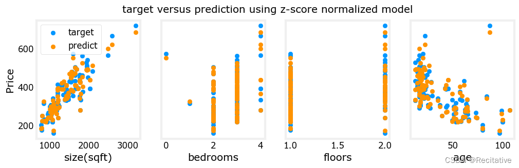
使用模型进行预测

y_pred_sgd = sgdr.predict(X_norm)

预测结果与目标值比对

Closed-form linear regression with scikit-learn

Scikit-learn 提供了闭式解线性回归模型linear regression model。具体推导可以参考Linear Regression & Gradient Descent这一节

线性回归闭式解本质上还是最小二乘。

linear regression model

Parameters:

• fit_interceptbool, default=True

  Whether to calculate the intercept for this model. If set to False, no intercept will be used in calculations (i.e. data is expected to be centered).

• copy_Xbool, default=True

  If True, X will be copied; else, it may be overwritten.

• n_jobsint, default=None

  The number of jobs to use for the computation. This will only provide speedup in case of sufficiently large problems, that is if firstly n_targets > 1 and secondly X is sparse or if positive is set to True. None means 1 unless in a joblib.parallel_backend context. -1 means using all processors. See Glossary for more details.

• positivebool, default=False

  When set to True, forces the coefficients to be positive. This option is only supported for dense arrays.New in version 0.24.

Attributes:

• **coef_**array of shape (n_features, ) or (n_targets, n_features)

  Estimated coefficients for the linear regression problem. If multiple targets are passed during the fit (y 2D), this is a 2D array of shape (n_targets, n_features), while if only one target is passed, this is a 1D array of length n_features.

• **rank_**int

  Rank of matrix X. Only available when X is dense.

• **singular_**array of shape (min(X, y),)

  Singular values of X. Only available when X is dense.

• **intercept_**float or array of shape (n_targets,)

  Independent term in the linear model. Set to 0.0 if fit_intercept = False.

• **n_features_in_**int

  Number of features seen during fit.New in version 0.24.

• **feature_names_in_**ndarray of shape (n_features_in_,)

  Names of features seen during fit. Defined only when X has feature names that are all strings.New in version 1.0.

fit the model

与之前不同的是，闭式解不需要对数据进行标准化。

创建并拟合模型

X_train, y_train = load_house_data()
linear_model = LinearRegression()
linear_model.fit(X_train, y_train) 

获取参数，进行预测

b = linear_model.intercept_
w = linear_model.coef_
x_house_predict = linear_model.predict(x_house)[0]

特征设计与多项式特征

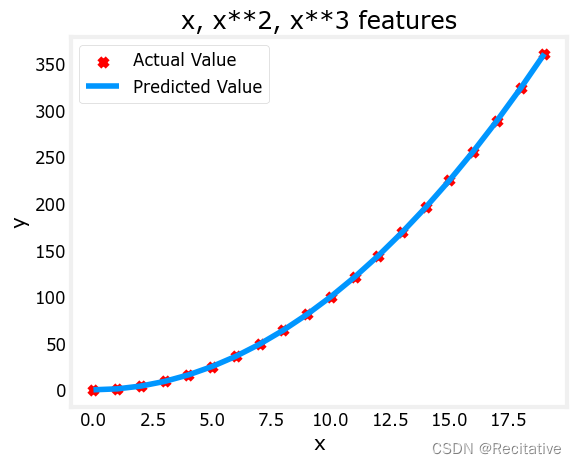
作为一点补充测试，尝试用scikit-learn处理下前面的多项式特征 创建数据

In [16]:

x = np.arange(0, 20, 1)
y = x**2

X = np.c_[x, x**2, x**3]

拟合模型

linear_model = LinearRegression()
linear_model.fit(X, y)

预测并绘图测试

model_w = linear_model.coef_
model_b = linear_model.intercept_
plt.scatter(x, y, marker='x', c='r', label="Actual Value"); plt.title("x, x**2, x**3 features")
plt.plot(x, X@model_w + model_b, label="Predicted Value"); plt.xlabel("x"); plt.ylabel("y"); plt.legend(); plt.show()